Download
1 / 175
1.77k likes | 1.95k Vues
THE HITCHHIKERS GUIDE TO POPULATION BALANCES, BREAK-UP AND COALESCENCE. Lecture series by: Lars Hagesaether October 2002. NTNU. Overview - START LECTURE 2. population balance to be solved in CFD-program:. function of break-up of ‘large’ particles. improved break-up model.

E N D
THE HITCHHIKERS GUIDE TO POPULATION BALANCES,BREAK-UP AND COALESCENCE. • Lecture series by: • Lars Hagesaether • October 2002 NTNU
Overview - START LECTURE 2 population balance to be solved in CFD-program: function of break-up of ‘large’ particles improved break-up model collision model for 2 fluid particles break-up for class i into class k collision frequency break-up probability
Overview OTHER MODELS BREAKUP MODEL COALESCENCE MODEL PB SIZE DISCRETIZATION CFD METHODS INPUT DATA COMBINED MODEL RESULTS • Note:.ppt file with lecture will be made available.
Population Balances Particle number continuity equation: Terms set to zero • For a sub-region, R, to move convectively with the particle phase-space velocity (i.e. Lagrangian viewpoint)
Population Balances • x is the set of internal and external coordinates (x, y, z) comprising the phase space R. • Since R can be any region, the integration parts can be removed thus giving the differential form of the number continuity equation in particle space. • Reference for equations above is Randolph & Larsson (1988)
By including the density and not including internal coordinates the transport equation for each class is: • Hagesæther (2002) and Hagesæther, Jakobsen & Svendsen (2000). Population Balances • It is also possible to use the Bolzmann transport equation as a starting point. • Time discretization by use of fractional time step method. The convective terms are calculated by use of an explicit second order method (a TVD scheme was used) • Berge & Jakobsen (1998) and Hagesæther (2002)
Birth and Death terms Coalescence: • Birth term collision phase film rupture (coalescence) • Death term • Death term Break-up: • Birth term collision phase break-up (uses energy) • Birth term • Death term
Birth and Death terms Column with coalescence and break-up: dispersed size distribution • figure from Chen, Reese & Fan (1994)
Birth and Death terms Coalescence example: Number of particles Dispersed Size Distribution • Death term • Death term • Birth term How to generate a finite (small) number of classes when coalescence and breakup can be between particles of any sizes? Volume
Birth and Death terms • Two methods for finite number of classes: • Interval size discretization • Hounslow, Ryall & Marshall (1988) and Litster, Smit & Hounslow (1995) • Finite point size discretization • Batterham, Hall & Barton (1981) and Hagesæther (2002) There are other methods beside population balances that may be used to solve the transport equation. These are not considered here.
Interval size discretization Equal volume example: Number of particles Dispersed Size Distribution First class Class covers an interval Volume, (length, area or ...)
Interval size discretization Coalescence example: Number of particles Dispersed Size Distribution • Death term • Death term • Birth term Which class does this one belong to? • 3 • 7 • 10 It should not matter as long as one is consistent Second example (problem illustrator) • 1 • 2 • 3 • 4 • 5 • 6 • 7 • 8 • 9 • 10 • 11 • 12 • 13 • 14 • 15 Volume
Interval size discretization Two possible classes for a new particle: • n + m - 1 • n • m • n + m Problem is how to differentiate between the two possibilities. Question: Does it matter?
Interval size discretization Answer: YES!, because if the class placement process of the new particles is done incorrectly it will lead to a systematic decrease or a systematic increase in the total mass of the system. (Easily seen if you assume that all particles are initially ‘center particles’)
2+2 3+3 7/10 3/4 5/6 6.5 9.5 7/10 8 Interval size discretization Example: 4 particles of classes 2, 2, 3 and 3, thus with initial masses of 1.5, 1.5, 2.5 and 2.5. Assume class 2 and class 2 coalescence, class 3 and class 3 coalescence, then coalescence between the two new particles. n+m-1 case gives a total mass decrease of 1.5 and n+m case gives a total mass increase of 1.5. Example n+m-1 n+m initial mass
Interval size discretization Suggestion: 50% to class n+m-1 and 50% to class n+m. This because a ‘center particle’ n and a ‘center particle’ m will give a particle on the border between classes n+m-1 and n+m. Evaluation: This is based on the assumption of (initial) flat profiles in the classes. Modifications are needed if class intervals varies in size. Conclusion: Suggested method must be tested and analytical tools for such testing are needed. Note: Same problem exist for the break-up case.
Interval size discretization Question: What physical properties do we want kept when using population balances, and why? • Some answers: • Number of particles, break-up is O(n) and coalescence is O(n2). • Length of particles, in crystallizing systems, though ‘McCabe L law’ assumes growth is not a function of length of the particle. • Area of particles, when diffusion is important. • Mass of particles, in CFD simulations. There may be other properties too...
Number of particles: • Assuming binary break-up and binary coalescence. • Compare this to sum of particles in classes. • Mass of particles: • Compare this to sum of mass in classes. Interval size discretization How to intuitively check if properties are kept: Note that length and area are more complicated, I do not know how to check these in a similar way...
Interval size discretization Scientific method - method of moments: average value for each class number in each class given on integral form and discrete form. Hounslow, Ryall & Marshall (1988) Zero moment:
Interval size discretization First moment: See also Edwards & Penney (1986) total length of particles weighted middle length of particles
Interval size discretization In general: number length area volume We now have a method for tracking either the total quantities or their average in the population balance system. Total volume (or mass) should be constant. How will the other quantities change with break-up and coalescence?
Interval size discretization I am not going to try to find such formulas. See Hounslow, Ryall & Marshall (1988). With only aggregation (coalescence) they get: well mixed batch system with constant volume. moment equation
Interval size discretization It is thus found that: collision frequency Thus it is found that the number of particles decrease with coalescence and that there is no change in the total volume. Discretization models should give the same result with the same assumptions
Discretization used: or Interval size discretization • Why Hounslow, Ryall & Marshall (1988)? • ‘Easy’ to understand this article. • ‘Standard’ reference for population balances. • Gives formulas for size discretization (coalescence). Number of particles • 1 • 2 • 3 • 4 Volume
Number of particles Volume, (length, area or ...) Interval size discretization Double volume intervals vs. equal sized intervals: Number of particles • Sometimes too few classes with this method Volume start of first interval must be set to > 0 • Generally dispersed particles are of several orders of magnitude • (for example 1 mm to 10 cm) • Mostly too many classes with this method
i-2 i-1 i i+1 Number of particles Volume Interval size discretization Definition of sizes in the system: Size of class i: Density in class i:
Interval size discretization • Mechanism for aggregation in interval i: • 1: i-1 and 1 to i-1 BIRTH • 2: i-1 and i-1 BIRTH • 3: i and 1 to i-1 DEATH • 4: i and i to infinity DEATH coalescence between
Interval size discretization • Details for mechanism 2, birth to class i: • 2: i-1 and i-1 BIRTH coalescence between i-1 i case one with maximum values Number of particles case two with minimum values Volume Both cases give a new fluid particle in class i. Thus, coalescence between any two particles of class i-1 gives a new fluid particle in class i.
Interval size discretization source term for mechanism number 2 coalescence frequency to avoid counting each coalescence twice - particle density in class i-1 The result above is also easily seen without the integration leading to it. The next mechanism is a bit more difficult.
Interval size discretization • Details for mechanism 1, birth to class i: • 1: i-1 and 1 to i-1 BIRTH minimum size needed of particle in interval i-1 to get the coalesced particle in class i. coalescence between i-2 i-1 i Number of particles Volume j class particle, j<i-1 Only a fraction of the coalescence between particle j and particles in class i-1 result in a particle in class i.
Interval size discretization i-2 i-1 i Number of particles Volume Number of particles available for coalescence: Above equation is based on an assumption, what is it? Even (or flat) distribution within each interval
Interval size discretization Next step is to integrate over the class the particle of size a belongs to coalescence frequency - particle density in class j Summing over all possible j classes gives
Interval size discretization • Details for mechanism 4, death of class i: • 4: i and i to infinity DEATH coalescence between case with minimum values i-1 i i+1 Number of particles Volume All possible coalescence cases result in the removal of a particle in class i.
Interval size discretization Integrate over j class gives Summing over all possible j classes gives When j=i, why is there no factor 0.5 included in order to avoid counting each coalescence twice? Trick question! It is included;) Also included is a factor 2 since two fluid particles are removed when i=j
Interval size discretization • Details for mechanism 3, death of class i: • 3: i and 1 to i-1 DEATH coalescence between minimum size needed of particle in interval i so that the new particle will be in class i+1. i-1 i i+1 Number of particles Volume j particle, j<i-1 Only a fraction of the coalescence between particle j and particles in class i result in the net removal of a particle from class i.
Interval size discretization Same as for mechanism 1, just writing up the final result Net rate of death for class i is thus given as: NOTE: factor k added to first and third terms Why is there a factor included?
Interval size discretization Why factor is added: same result for any value of factor k ONLY when k = 2/3
Interval size discretization • Summary for Hounslow et al. (1988) article: • Geometric interval size discretization given • Factor 2 between each class • Aggregation (coalescence) formula given • Nucleation and growth also formulated • Number balance and mass balance satisfied • Assumes flat distribution in each class • Generally good results with model used • Break-up not included
Interval size discretization • Further reading material: • Litster, Smit & Hounslow (1995) give a refined geometric model for aggregation and growth where • Hill & Ng (1995) give a discretization procedure for the breakage equation, allowing any geometric ratio. • Kostoglou & Karabelas (1994) and Vanni (2000) test several size discretization schemes on several test cases. whole positive integer
Finite point size discretization • Some literature for finite point size discretization: • Batterham, Hall & Barton (1981), first to use finite point size discretization. They made a mistake in their balance though, see Hounslow, Ryall & Marshall (1988) • Kumar & Ramkrishna (1996). Article series starting with this one. • Ramkrishna (2000). Book about population balances in general. No more details here than in the article series.
Finite point size discretization • Own methods for finite point size discretization: • Geometric factor 2 increase • Randomly increasing class sizes Will show both versions, starting with the first one since that one is simplest (easiest).
Geometric factor 2 increase Discretization used: Only fluid particles with these exact sizes are allowed What should be done with a fluid particle in this area? Number of particles mass • 1 • 2 • 3 • 4
Geometric factor 2 increase Particle between two classes: divide particle into classes i and i+1 How to divide the particle into the two bounding allowed sizes?
Geometric factor 2 increase Mass balance: mass of particle number density of particle Number balance: Combined: the only unknown variable With number balance and mass balance used there is only one possible split between the classes for each case
Geometric factor 2 increase Break-up into two daughter fragments with the smallest fragment of a population class size: largest daughter particle Model requires that smallest daughter fluid particle is of a population class size, thus k<i. Model requires break-up into two daughter fragments.
Geometric factor 2 increase Break-up: largest daughter particle is split into two classes Why is fragment above split into classes i-1 and i? Largest fragment must be at least half the mass of the parent particle. Half the mass of the parent particle is the mass of the class below. Thus the largest fragment must be in the interval between classes i-1 and i. ‘x’ is given by the mass balance and the number balance parent class daughter class
Geometric factor 2 increase Details for particle balance class splitting Using Giving
Geometric factor 2 increase Coalescence of two particles: Coalescence: largest parent particle found same way as for break-up parent class parent class The largest parent particle is defined with index i
total break-up rate, Geometric factor 2 increase What are the break-up rates? smallest daughter parent particle volume balance gives: second daughter particle Number of particles mass • 1 • 2 • 3 • 4
total break-up rate, Geometric factor 2 increase Finding break-up source terms by use of a test case: If 4 classes, the possible break-ups are: parent class smallest daughter class parent class Example: amount breaking up of class 4 into class 3 total amount into class 3 from splitting the largest particle