Download
1 / 42
440 likes | 676 Vues
Applied Cartography and Introduction to GIS GEOG 2017 EL. Lecture-7 Chapters 13 and 14. Data for Terrain Mapping and Analysis. DEM (digital elevation model) and TIN (triangulated irregular network) are two common types of input data for terrain mapping and analysis.

E N D
Applied Cartography and Introduction to GISGEOG 2017 EL Lecture-7 Chapters 13 and 14
Data for Terrain Mapping and Analysis • DEM (digital elevation model) and TIN (triangulated irregular network) are two common types of input data for terrain mapping and analysis. • A DEM represents a regular array of elevation points. It can be converted to an elevation raster by placing each elevation point at the center of a cell. • A TIN approximates the land surface with a series of nonoverlapping triangles.
Raster/TIN Conversion • The maximum z-tolerance algorithm selects points from an elevation raster to construct a TIN such that, for every point in the elevation raster, the difference between the original elevation and the estimated elevation from the TIN is within the specified maximum z-tolerance. • A TIN can be converted into a DEM by using local first-order polynomial interpolation.
Input Data to TIN Besides DEM, a TIN can also use additional point data such as surveyed elevation points, GPS (global positioning system) data, and LIDAR data; line data such as contour lines and breaklines; and area data such as lakes and reservoirs.
Breakline A breakline, shown as a dashed line in (b), subdivides the triangles in (a) into a series of smaller triangles in (c).
Terrain Mapping Terrain mapping techniques include contouring, vertical profiling, hill shading, hypsometric tinting, and perspective view.
Hill Shading An example of hill shading, with the sun’s azimuth at 315° (NW) and the sun’s altitude at 45°.
Hypsometric Map A hypsometric map. Different elevation zones are shown in different gray symbols.
3D View Three controlling parameters of the appearance of a 3-D view: the viewing azimuth a is measured clockwise from the north, the viewing angle u is measured from the horizon, and the viewing distance d is measured between the observation point and the 3-D surface.
Draping Draping of streams and shorelines on a 3-D surface.
Slope and Aspect • Slopemeasures the rate of change of elevation at a surface location. Slope may be expressed as percent slope or degree slope. • Aspect is the directional measure of slope. Aspect starts with 0° at the north, moves clockwise, and ends with 360° also at the north. Because it is a circular measure, We often have to manipulate aspect measures before using them in data analysis.
Slope Measurement Slope, either measured in percent or degrees, can be calculated from the vertical distance a and the horizontal distance b.
Aspect Measures Aspect measures are often grouped into the four principal directions (top) or eight principal directions (bottom).
Computing Algorithms for Slope and Aspect Using Raster • The slope and aspect for an area unit (i.e., a cell or triangle) are measured by the quantity and direction of tilt of the unit’s normal vector—a directed line perpendicular to the unit. • Different approximation (finite difference) methods have been proposed for calculating slope and aspect from an elevation raster. Usually based on a 3-by-3 moving window, these methods differ in the number of neighboring cells used in the estimation and the weight applying to each cell.
Slope and Aspect The normal vector to the cell is the directed line perpendicular to the cell. The quantity and direction of tilt of the normal vector determine the slope and aspect of the cell.
Computing Algorithms for Slope and Aspect using TIN The x, y, and z values of points that make up a TIN are used to compute slope and aspect for each triangle. The algorithm for computing slope and aspect of a triangle in a TIN uses the x, y, and z values at the three nodes of the triangle.
Factors Influencing Slope and Aspect Measures Factors that can influence slope and aspect measures include the resolution of DEM, the quality of DEM, the computing algorithm, and local topography.
DEM DEMs at three different resolutions: USGS 30-meter DEM (a), USGS 10-meter DEM (b), and 1.83-meter DEM derived from LIDAR data (c).
Viewshed Analysis A viewshedrefers to the portion of the land surface that is visible from one or more viewpoints. The process for deriving viewsheds is called viewshed or visibility analysis.
Line-Of-Sight Operation • The line-of-sight operation is the basis for viewshed analysis. • The line of sight connects the viewpoint and the target. If any land, or any object on the land, rises above the line, then the target is invisible to the viewpoint. If no land or object blocks the view, then the target is visible to the viewpoint.
Sightline A sightline connects two points on a TIN in (a). The vertical profile of the sightline is depicted in (b). In both diagrams, the visible portion is shown in white and the invisible portion in black.
Cumulative Viewshed • The output of a viewshed analysis is a binary map showing visible and not visible areas. • Given one viewpoint, a viewshed map has the value of 1 for visible and 0 for not visible. • Given two or more viewpoints, a viewshed map becomes a cumulative viewshed map. Two options are common for presenting a cumulative viewshed map. The first option uses counting operations, with the number of possible values being (the number of viewpoints) + 1. The second option uses Boolean operations.
Cumulative Viewshed Map Two options for presenting a cumulative viewshed map: the counting option (a) and the Boolean option (b).
Accuracy of Viewshed Analysis • The accuracy of viewshed analysis depends on the accuracy of the surface data, the data model (i.e., TIN versus DEM), and the rule for judging visibility. • Some researchers have suggested that visibility be expressed in probabilistic, rather than binary, terms.
Parameters of Viewshed Analysis A number of parameters can influence the result of a viewshed analysis including the viewpoint, the height of the observer, the viewing azimuth, the viewing radius, vertical viewing angle limits, the Earth’s curvature, and tree height.
The increase of the visible areas from (a) to (b) is a direct result of adding 20 meters to the height of the viewpoint.
The difference in the visible areas between (a) and (b) is due to the viewing angle: 00 to 3600 in (a) and 00 to 1800 in (b).
The difference in the visible areas between (a) and (b) is due to the search radius: infinity in (a) and 8000 meters from the viewpoint in (b).
Watershed Analysis • A watershedrefers to an area, defined by topographic divides, that drains surface water to a common outlet. • A watershed is often used as a unit area for the management and planning of water and other natural resources. • Watershed analysisrefers to the process of using DEMs and following water flows to delineate stream networks and watersheds.
Delineation of Watersheds • Delineation of watersheds can take place at different spatial scales. • Delineation of watersheds can also be area-based or point-based. An area-based method divides a study area into a series of watersheds, one for each stream section. A point-based method derives a watershed for each select point.
Steps for automated watershed Delineation • Make a filled DEM. • Derive a flow direction raster, which shows the direction water will flow out of each cell. • Derive a flow accumulation raster, which tabulates for each cell the number of cells that will flow to it. • Derive a stream network by applying a threshold value to a flow accumulation raster. • Derive stream links, with each link assigned a unique value and a flow direction. • Delineate watershed by using the flow direction raster and the stream link raster as the inputs.
This illustration shows a filled elevation raster (a), a flow direction raster (b), and a flow accumulation raster (c). Both shaded cells in (c) have the same flow accumulation value of 2. The top cell receives its flow from its left and lower-left cells. The bottom cell receives its flow from its lower-left cell, which already has a flow accumulation value of 1.
A flow accumulation raster, with darker symbols representing higher flow accumulation values.
To derive the stream links, each section of the stream network is assigned a unique value and a flow direction. The inset map on the right shows three stream links.
A stream link raster includes reaches, junctions, flow directions, and an outlet.
Point-Based Watersheds Point-based watersheds have one watershed associated with each point, which may be a stream gage station, a dam, or a surface drinking water system intake location. In watershed analysis, these points of interest are called pour points or outlets.
Snap a Pour Point • If a pour point is not located directly over a stream link, it will result in a small, incomplete watershed for the outlet. • The solution is to use a command to snap a pour point to a stream cell within a user-defined search radius.
If a pour point (black circle) is not snapped to a cell with a high flow accumulation value (dark cell symbol), it usually has a small number of cells (shaded area) identified as its watershed.
Algorithm for Deriving a Point-Based Watershed • If the pour point is located at a junction, then the watersheds upstream from the junction are merged to form the watershed for the pour point. • If the pour point is located between two junctions, then the watershed assigned to the stream section between the two junctions is divided into two, one upstream from the pour point and the other downstream. The upstream portion of the watershed is then merged with watersheds further upstream to form the watershed for the pour point.
Factors Influencing Watershed Analysis Factors influencing the outcome of a watershed analysis include DEM resolution, flow direction method, and flow accumulation threshold. DEMs at a 30-meter resolution (a) and a 10-meter resolution (b).
Stream networks derived from the DEMs in Figure 14.20. The stream network derived from the 30-meter DEM (a) has fewer details than that from the 10-meter DEM (b).