Classical scheduling algorithms for periodic systems

1. Classical scheduling algorithmsfor periodic systems Peter Marwedel TU Dortmund, Informatik 12 Germany 2007/12/14

2. Structure of this course guest lecture on multisensor systems (Fink) New clustering 3: Embedded System HW 5: Scheduling,HW/SW-Partitioning, Applications to MP-Mapping 2: Specifications 8: Testing Application Knowledge 4: Standard Software, Real-Time Operating Systems 7: Optimization of Embedded Systems 6: Evaluation guest lecture from industry (NXP) [Digression: Standard Optimization Techniques (1 Lecture)] guest lecture on (RT-) OS (Spinczyk)

3. Classes of mapping algorithmsconsidered in this course • Classical scheduling algorithmsMostly for independent tasks & ignoring communication, mostly for mono- and homogeneous multiprocessors • Hardware/software partitioningDependent tasks, heterogeneous systems,focus on resource assignment • Dependent tasks as considered in architectural synthesisInitially designed in different context, but applicable • Design space exploration using genetic algorithmsHeterogeneous systems, incl. communication modeling

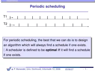
4. Periodic scheduling • For periodic scheduling, the best that we can do is to design an algorithm which will always find a schedule if one exists. A scheduler is defined to be optimal iff it will find a schedule if one exists. T1 T2

5. Periodic scheduling • Let • pi be the period of task Ti, • ci be the execution time of Ti, • dibe the deadline interval, that is, the time between a job ofTi becoming available and the time until the same job Ti has to finish execution. • ℓi be the laxity or slack, defined asℓi= di - ci pi di ci ℓi

6. Accumulated utilization • Accumulated utilization: Necessary condition for schedulability(with m=number of processors):

7. Independent tasks:Rate monotonic (RM) scheduling • Most well-known technique for scheduling independent • periodic tasks [Liu, 1973]. • Assumptions: • All tasks that have hard deadlines are periodic. • All tasks are independent. • di=pi, for all tasks. • ci is constant and is known for all tasks. • The time required for context switching is negligible. • For a single processor and for n tasks, the following equation holds for the accumulated utilization µ:

8. Rate monotonic (RM) scheduling- The policy - RM policy: The priority of a task is a monotonically decreasing function of its period. At any time, a highest priority task among all those that are ready for execution is allocated. Theorem: If all RM assumptions are met, schedulability is guaranteed.

9. Maximum utilization for guaranteed schedulability Maximum utilization as a function of the number of tasks:

10. Example of RM-generated schedule T1 preempts T2 and T3. T2 and T3 do not preempt each other.

11. Case of failing RM scheduling Task 1: period 5, execution time 2 Task 2: period 7, execution time 4 µ=2/5+4/7=34/35  0.97 2(21/2-1)  0.828 Missing computations scheduled in the next period Missed deadline

12. Intuitively: Why does RM fail ? No problem if p2 = m p1, mℕ : Switching to T1 too early, despite early deadline for T2 T1 t T2 should be completed T1 fits t T2 leviRTS animation

13. Morein-depth: Proof of RM optimality • Definition: A critical instant of a task is the time at which the release of a task will produce the largest response time. • Lemma: For any task, the critical instant occurs if that task is simultaneously released with all higher priority tasks. • Proof: Let T={T1, …,Tn}: periodic tasks with i: pi ≦ pi +1. Source: G. Buttazzo, Hard Real-time Computing Systems, Kluwer, 2002

14. Critical instances (1) • Response time of Tn is delayed by tasks Tiof higher priority: Tn Ti t cn+2ci • Delay may increase if Ti starts earlier Tn Ti t cn+3ci • Maximum delay achieved if Tn and Ti start simultaneously.

15. Critical instances (2) • Repeating the argument for all i = 1, … n-1: • The worst case response time of a task occurs when it is released simultaneously with all higher-priority tasks. q.e.d. • Schedulability is checked at the critical instants. • If all tasks of a task set are schedulable at their critical instants, they are schedulable at all release times.

16. The case i:pi+1 = mi pi • Lemma*: If each task period is a multiple of the period of the next higher priority task, then schedulability is also guaranteed if µ  1. • Proof: Assume schedule of Ti is given. Incorporate Ti+1: Ti+1 fills idle times of Ti; Ti+1 completes in time, if µ  1. Ti Ti+1 t  T’i+1 Used as the higher priority task at the next iteration. * wrong in the book

17. Proof of the RM theorem • Let T={T1, T2} with p1 < p2. • Assume RM is notused  prio(T2) is highest: p1 T1 c1 T2 t c2 • Schedule is feasible if c1+c2≦ p1 (1) • Define F= p2/p1: # of periods of T1fully contained in T2

18. Case 1: c1p2 – Fp1 • Assume RM is used  prio(T1) is highest: • Case 1*: c1p2 – Fp1(c1 small enough to be finished before 2nd instance of T2) T1 T2 t Fp1 p2 • Schedulable if (F+1) c1 + c2p2 (2) * Typos in [Buttazzo 2002]: < and  mixed up]

19. Proof of the RM theorem (3) • Not RM: schedule is feasible if c1+c2p1 (1) • RM: schedulable if (F+1) c1 + c2p2 (2) • From (1): Fc1+Fc2Fp1 • Since F  1: Fc1+c2  Fc1+Fc2Fp1 • Adding c1: (F+1)c1+c2 Fp1 +c1 • Since c1p2 – Fp1: (F+1)c1+c2 Fp1 +c1 p2 • Hence: if (1) holds, (2) holds as well • For case 1: Given tasks T1 and T2 with p1 < p2, then if the schedule is feasible by an arbitrary (but fixed) priority assignment, it is also feasible by RM.

20. Case 2: c1>p2 – Fp1 • Case 2: c1>p2 – Fp1(c1 large enough not to finish before 2nd instance of T2) T1 T2 t Fp1 p2 • Schedulable if F c1 + c2F p1 (3) • c1+c2p1 (1) • Multiplying (1) by F yields Fc1+ F c2Fp1 • Since F  1: Fc1+ c2 Fc1+ Fc2Fp1 •  Same statement as for case 1.

21. Calculation of the least upper utilization bound • Let T={T1, T2} with p1 < p2. • Proof procedure: compute least upper bound Ulup as follows • Assign priorities according to RM • Compute upper bound Uup by setting computation times to fully utilize processor • Minimize upper bound with respect to other task parameters • As before: F= p2/p1 • c2 adjusted to fully utilize processor.

22. Case 1: c1p2 – Fp1 • Largest possible value of c2 is c2= p2 – c1 (F+1) • Corresponding upper bound is T1 T2 t Fp1 p2 { } is <0  Uub monotonically decreasing in c1 Minimum occurs for c1 = p2 – Fp1

23. Case 2: c1p2 – Fp1 • Largest possible value of c2 is c2= (p1-c1)F • Corresponding upper bound is: T1 T2 t Fp1 p2 { } is  0  Uub monotonically increasing in c1 (independent of c1 if {}=0) Minimum occurs for c1 = p2 – Fp1, as before.

24. Utilization as a function of G=p2/p1-F • For minimum value of c1: Since 0 G< 1: G(1-G)  0  Uub increasing in F  Minimum of Uub for min(F): F=1 

25. end Proving the RM theorem for n=2 • This proves the RM theorem for the special case of n=2

26. Properties of RM scheduling • RM scheduling is based on static priorities. This allows RM scheduling to be used in standard OS, such as Windows NT. • No idle capacity is needed if i: pi+1=F pi: i.e. if the period of each task is a multiple of the period of the next higher priority task, schedulability is then also guaranteed if µ  1. • A huge number of variations of RM scheduling exists. • In the context of RM scheduling, many formal proofs exist.

27. EDF • EDF can also be applied to periodic scheduling. • EDF optimal for every period • Optimal for periodic scheduling • EDF must be able to schedule the example in which RMS failed.

28. Comparison EDF/RMS • RMS: EDF: T2 not preempted, due to its earlier deadline. EDF-animation

29. EDF: Properties • EDF requires dynamic priorities •  EDF cannot be used with a standard operating system just providing static priorities.

30. Comparison RMS/EDF

31. Sporadic tasks • If sporadic tasks were connected to interrupts, the execution • time of other tasks would become very unpredictable. •  Introduction of a sporadic task server,periodically checking for ready sporadic tasks; •  Sporadic tasks are essentially turned into periodic tasks.

32. Dependent tasks • Strategies: • Add resources, so that scheduling becomes easier • Split problem into static and dynamic part so that only a minimum of decisions need to be taken at run-time. • Use scheduling algorithms from high-level synthesis The problem of deciding whether or not a schedule existsfor a set of dependent tasks and a given deadlineis NP-complete in general [Garey/Johnson].

33. Summary • Periodic scheduling • Rate monotonic scheduling • Proof of the utilization bound for n=2. • EDF • Dependent and sporadic tasks (briefly)