Analyzing ARIMA Models: Fitting, Estimation, and Forecasting Techniques
This document discusses the modelling of time series data using ARIMA approaches. It outlines the identification process through the examination of the Sample Autocorrelation (SAC) and Sample Partial Autocorrelation (SPAC) functions, suggesting an AR(1) model as a fit. It emphasizes the importance of Maximum Likelihood over Least-Squares estimation methods due to varying response and explanatory variables. Additionally, it includes iterations for parameter estimation, diagnostics using the Ljung-Box test, and considerations for AR(p) and MA(q) models, addressing residual correlation and forecasts.

Analyzing ARIMA Models: Fitting, Estimation, and Forecasting Techniques
E N D
Presentation Transcript
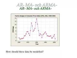
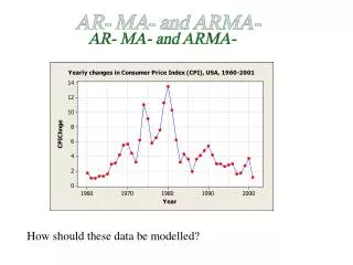
AR- MA- and ARMA- How should these data be modelled?
Identification step: Look at the SAC and SPAC Looks like an AR(1)-process. (Spikes are clearly decreasing in SAC and there is maybe only one sign. spike in SPAC)
Then we should try to fit the model The parameters to be estimated are and . One possibility might be to uses Least-Squares estimation (like for ordinary regression analysis) Not so wise, as both response and explanatory variable are randomly varying. Maximum Likelihood better So-called Conditional Least-Squares method can be derived Use MINITAB’s ARIMA-procedure!!
AR(1) We can always ask for forecasts
MTB > ARIMA 1 0 0 'CPIChnge'; SUBC> Constant; SUBC> Forecast 2 ; SUBC> GSeries; SUBC> GACF; SUBC> GPACF; SUBC> Brief 2. ARIMA Model: CPIChnge Estimates at each iteration Iteration SSE Parameters 0 316.054 0.100 4.048 1 245.915 0.250 3.358 2 191.627 0.400 2.669 3 153.195 0.550 1.980 4 130.623 0.700 1.292 5 123.976 0.820 0.739 6 123.786 0.833 0.645 7 123.779 0.836 0.626 8 123.778 0.837 0.622 9 123.778 0.837 0.621 Relative change in each estimate less than 0.0010
Final Estimates of Parameters Type Coef SE Coef T P AR 1 0.8369 0.0916 9.13 0.000 Constant 0.6211 0.2761 2.25 0.030 Mean 3.809 1.693 Number of observations: 42 Residuals: SS = 122.845 (backforecasts excluded) MS = 3.071 DF = 40
All spikes should be within red limits here, i.e. no correlation should be left in the residuals!
Modified Box-Pierce (Ljung-Box) Chi-Square statistic Lag 12 24 36 48 Chi-Square 26.0 35.3 39.8 * DF 10 22 34 * P-Value 0.004 0.036 0.227 * Forecasts from period 42 95% Limits Period Forecast Lower Upper Actual 43 1.54176 -1.89376 4.97727 44 1.91148 -2.56850 6.39146
Ljung-Box statistic: where n is the sample size d is the degree of non-seasonal differencing used to transform original series to be stationary. Non-seasonal means taking differences at lags nearby. rl2(â) is the sample autocorrelation at lag l for the residuals of the estimated model. K is a number of lags covering multiples of seasonal cycles, e.g. 12, 24, 36,… for monthly data
Under the assumption of no correlation left in the residuals the Ljung-Box statistic is chi-square distributed with K – nC degrees of freedom, where nC is the number of estimated parameters in model except for the constant • A low P-value for any K should be taken as evidence for correlated residuals, and thus the estimated model must be revised. In this example: Here, data is not supposed to possess seasonal variation so interest is mostly paid to K = 12. P – value for K =12 is lower than 0.05 Model needs revision! Modified Box-Pierce (Ljung-Box) Chi-Square statistic Lag 12 24 36 48 Chi-Square 26.0 35.3 39.8 * DF 10 22 34 * P-Value 0.004 0.036 0.227 * K
A new look at the SAC and SPAC of original data: • The second spike in SPAC might be considered crucial! • If an AR(p)-model is correct, the ACF should decrease exponentially (monotonically or oscillating) • and PACF should have exactly p significant spikes • Try an AR(2) i.e.
Type Coef SE Coef T P AR 1 1.1684 0.1509 7.74 0.000 AR 2 -0.4120 0.1508 -2.73 0.009 Constant 1.0079 0.2531 3.98 0.000 Mean 4.137 1.039 Number of observations: 42 Residuals: SS = 103.852 (backforecasts excluded) MS = 2.663 DF = 39 Modified Box-Pierce (Ljung-Box) Chi-Square statistic Lag 12 24 36 48 Chi-Square 18.6 30.6 36.8 * DF 9 21 33 * P-Value 0.029 0.081 0.297 * Forecasts from period 42 95% Limits Period Forecast Lower Upper Actual 43 0.76866 -2.43037 3.96769 44 1.45276 -3.46705 6.37257 PREVIOUS MODEL: Residuals: SS = 122.845 (backforecasts excluded) MS = 3.071 DF = 40 Modified Box-Pierce (Ljung-Box) Chi-Square statistic Lag 12 24 36 48 Chi-Square 26.0 35.3 39.8 * DF 10 22 34 * P-Value 0.004 0.036 0.227 * Forecasts from period 42 95% Limits Period Forecast Lower Upper Actual 43 1.54176 -1.89376 4.97727 44 1.91148 -2.56850 6.39146
Could it be the case of an Moving Average (MA) model? MA(1): {at}are still assumed to be uncorrelated and identically distributed with mean zero and constant variance
MA(q): • always stationary • mean = • is in effect a moving average with weights for the (unobserved) values at, at – 1, … , at – q
Final Estimates of Parameters Type Coef SE Coef T P MA 1 -1.0459 0.0205 -51.08 0.000 Constant 4.5995 0.3438 13.38 0.000 Mean 4.5995 0.3438 Number of observations: 42 Residuals: SS = 115.337 (backforecasts excluded) MS = 2.883 DF = 40 Modified Box-Pierce (Ljung-Box) Chi-Square statistic Lag 12 24 36 48 Chi-Square 38.3 92.0 102.2 * DF 10 22 34 * P-Value 0.000 0.000 0.000 * Forecasts from period 42 95% Limits Period Forecast Lower Upper Actual 43 1.27305 -2.05583 4.60194 44 4.59948 -0.21761 9.41656 Not at all good! Much wider!
Still seems to be problems with residuals Look again at ACF and PACF of original series: The pattern corresponds neither with pure AR(p), nor with pure MA(q) Could it be a combination of these two? Auto Regressive Moving Average (ARMA) model
ARMA(p,q): • stationarity conditions harder to define • mean value calculations more difficult • identification patterns exist, but might be complex: • exponentially decreasing patterns or • sinusoidal decreasing patterns in both ACF and PACF (no cutting of at a certain lag)
Always try to keep p and q small. Try an ARMA(1,1):
Type Coef SE Coef T P AR 1 0.6558 0.1330 4.93 0.000 MA 1 -0.9324 0.0878 -10.62 0.000 Constant 1.3778 0.4232 3.26 0.002 Mean 4.003 1.230 Number of observations: 42 Residuals: SS = 77.6457 (backforecasts excluded) MS = 1.9909 DF = 39 Modified Box-Pierce (Ljung-Box) Chi-Square statistic Lag 12 24 36 48 Chi-Square 8.4 21.5 28.3 * DF 9 21 33 * P-Value 0.492 0.429 0.699 * Forecasts from period 42 95% Limits Period Forecast Lower Upper Actual 43 -1.01290 -3.77902 1.75321 44 0.71356 -4.47782 5.90494 Much better!
Calculating forecasts For AR(p) models quite simple: at + kis set to 0 for all values of k
For MA(q) ?? MA(1): If we e.g. would set at and at – 1 equal to 0 the forecast would constantly be which is not desirable.
Note that Similar investigations for ARMA-models.