CS 201 Data Structures and Algorithms

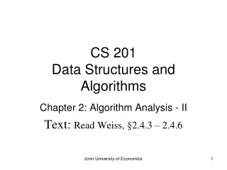
1. CS 201Data Structures and Algorithms Chapter 4: Trees (BST) Text: Read Weiss, §4.3 Izmir University of Economics

2. The Search Tree ADT – Binary Search Trees • An important application of binary trees isin searching.Let us assume that each node in the tree stores an item. Assume for simplicity that these are distinct integers (deal with duplicates later). • The property that makes a binary tree into a binary search tree is that for every node, X, in the tree, the values of all the items in the left subtree are smaller than the item in X, and the values of items in the right subtree are larger than the item in X. The tree on the left is a binary search tree, but the tree on the right is not. The tree on the right has a node with key 7 in the left subtree of a node with key 6 (which happens to be the root). Izmir University of Economics

3. Binary Search Trees - Operations • Descriptions and implementations of theoperations that are usually performed on binary search trees (BST) are given. • Note that because of the recursive definition of trees, it is common to write these routines recursively. Because the average depth of a binary search tree is O(log N), we generally do not need to worry about running out of stack space. • Since all the elements can be ordered, we will assume that the operators <, >, and = can be applied to them. Izmir University of Economics

4. BST – Implementation - I typedef int ElementType; struct TreeNode; typedef struct TreeNode *Position; typedef struct TreeNode *SearchTree; struct TreeNode{ ElementType Element; SearchTree Left; SearchTree Right; }; SearchTree MakeEmpty(SearchTree T){ if( T != NULL ){ MakeEmpty( T->Left ); MakeEmpty( T->Right ); free( T ); } return NULL; } Notice that NULL is returned at the end. Izmir University of Economics

5. BST – Implementation - II • Findoperation generally requires returning a pointer to the node in the Binary Search Tree pointed byT that has value X, or NULL if there is no such node. The structure of the tree makes this simple. If T is NULL , then we can just return .Otherwise, we make a recursive call on either the left or the rightsubtree of the node pointed byT,depending on the relationship of X to the value stored in the node pointed byT. Otherwise, if the value stored X, we can return T. Position Find(ElementType X, SearchTree T){ if( T == NULL ) return NULL; if( X < T->Element ) return Find( X, T->Left ); else if( X > T->Element ) return Find( X, T->Right ); else return T; } Izmir University of Economics

6. BST – Implementation - III • To perform a FindMin, start at the root and go left as long as there is a left child. The stopping point is the smallest element. • The FindMax routine is the same, except that branching is to the right child. • Notice that the degenerate case of an empty tree is carefully handled. • Also notice that it is safe to change T in FindMax, since we are only working with a copy. Always be extremely careful, however, because a statement such as • T->right=T->right->right will make changes. Position FindMin(SearchTree T){ if( T == NULL ) return NULL; else if( T->Left == NULL ) return T; else return FindMin( T->Left ); } Position FindMax(SearchTree T){ if( T != NULL ) while( T->Right != NULL ) T = T->Right; return T; } Izmir University of Economics

7. BST – Implementation – Insertion I The insertion routine is conceptually simple. To insert X into tree T, proceed down the tree as you would with a Find. If X is found, do nothing (or "update" something). Otherwise, insert X at the last spot on the path traversed.Duplicates can be handled by keeping an extra field in the node indicating the frequency of occurrence. If the key is only part of a larger record, then all of the records with the same key might be kept in an auxiliary data structure, such as a list or another search tree. → Insert node 5 Izmir University of Economics

8. BST – Implementation – Insertion II SearchTree Insert(ElementType X, SearchTree T){ if( T == NULL ){ /* Create and return a one-node tree */ T = malloc( sizeof( structTreeNode ) ); if( T == NULL ) FatalError( "Out of space!!!" ); else { T->Element = X; T->Left = T->Right = NULL; } } else if( X < T->Element ) T->Left = Insert( X, T->Left ); else if( X > T->Element ) T->Right = Insert( X, T->Right ); /* Else X is in the tree already; do nothing */ return T; /* Do not forget this line!! */ } Izmir University of Economics

9. BST – Implementation – Deletion I • Once we have found the node to be deleted, we need to consider 3 possibilities. (1)If the node is a leaf, it can be deleted immediately. (2)If the node has one child, the node can be deleted after its parent adjusts a pointer to bypass the node.Notice that the deleted node is now unreferenced and can be disposed of only if a pointer to it has been saved. → Delete node 4 Izmir University of Economics

10. BST – Implementation – Deletion II (3) The complicated case deals with a node with two children. The general strategy is to replace the key of this node with the smallest key of the right subtree (easy) and recursively delete that node (which is now empty). Because the smallest node in the right subtree cannot have a left child, the second delete is an easy one. → Delete node 2 Izmir University of Economics

11. BST – Implementation – Deletion III SearchTree Delete(ElementType X, SearchTree T){ Position TmpCell; /* declare a pointer */ if( T == NULL ) Error( "Element not found" ); else if( X < T->Element ) /* Go left */ T->Left = Delete( X, T->Left ); else if( X > T->Element ) /* Go right */ T->Right = Delete( X, T->Right ); elseif( T->Left && T->Right ){/* Found, it has 2 children */ TmpCell = FindMin( T->Right ); /* smallest in the right */ T->Element = TmpCell->Element; /* Replace with smallest */ T->Right = Delete( T->Element, T->Right ); } else {/* Found, it has one or zero children */ TmpCell = T; T = (T->Left)?T->Left:T->Right;/* Also handles 0 children */ free( TmpCell ); } return T; } Inefficient, since calls highlighted in yellow result in two passes downthe tree to find and deletethe smallestnode inthe right subtree. Izmir University of Economics

12. BST – Implementation – Deletion IV SearchTree Delete(ElementType X, SearchTree T){ Position TmpCell, TmpPrevCell;/* declare another pointer */ ... elseif( T->Left && T->Right ){ /* Found, it has 2 children */ TmpCell = T->Right; /* to point to smallest in the right */ TmpPrevCell = T->Right; /* to point to parent of TmpCell */ while (TmpCell->Left != NULL){/* find smallest of right */ TmpPrevCell = TmpCell; TmpCell = TmpCell->Left; } T->Element = TmpCell->Element;/* replace with smallest */ if (TmpCell == TmpPrevCell)/* T->Right is smallest */ T->Right = TmpCell->Right;/* skip over TmpCell */ else /* connect Left of TmpPrevCell to Right of TmpCell */ TmpPrevCell->Left = TmpCell->Right; free (TmpCell); } ... } • We can use stacks to convert an expression in standart form (otherwise known as infix) into postfix. • Example: operators = {+, *, (, )}, usual precedence rules; a + b * c + (d * e + f) * g Answer = a b c * + d e * f + g * + Efficient Version Izmir University of Economics

13. BST – Implementation – Lazy Deletion • If the number of deletions is small, then a popular strategy to use is lazy deletion: When an element is to be deleted, it is left in the tree and merely marked as deleted.This is especially popular if duplicates are present, because then the field that keeps count of the items can be decremented. • If the number of real nodes is the same as the number of "deleted" nodes, then the depth of the tree is only expected to go up by a small constant (why?), so there is a very small time penalty associated with lazy deletion. Also, if an item is reinserted, the overhead of allocating a new cell is avoided. Izmir University of Economics

14. Average-Case Analysis - I • All of the operations of BST, except MakeEmpty, take O(d) timewhere d is the depth of the node containing the accessed key. As a result, they are O (depth of tree). • Why?Because in constant time we descend a level in the tree, thus operating on a tree that is now roughly half as large. • MakeEmpty take O(N) time. • Observation: The average depth over all nodes in a BST is O(log N) assuming all insertion sequences are equally likely. • Proof: The sum of the depths of all nodes in a tree is the internal path length. Let’s calculate the average internal path length over all possible insertion sequences. Izmir University of Economics

15. Average-Case Analysis - II • Let D(N) be the internal path length for some BST T of N nodes. D(1) = 0. • D(N) = D(i) + D(N-i-1) + N -1 // Subtree nodes are 1 level deeper • All subtree sizes are equally likely for BSTs, since it depends only on the rank of the first element inserted into BST. This does not hold for binary trees though. Let’s, then, average: • If the recurrence is solved, D(N) = O(N log N). Thus, the expected depth of any node is O(log N). Izmir University of Economics

16. Derivation of D(N) - 1 .....(subtract (2) from (1)) .....(divide by N(N+1)) ...(sum the equations side by side) Izmir University of Economics

17. Derivation of D(N) - 2 Izmir University of Economics

18. Average-Case Analysis - III • As an example, the randomly generated 500 node BST has nodes at expected depth 9.98. Izmir University of Economics

19. Average-Case Analysis - IV • Deletion algorithm described favors making left subtrees deeper than the right (a deleted node is replaced with a node from the right). The exact effect of this still unknown, but if insertions and deletions are alternated Ɵ(N2) times, expected depth is .In the absence of deletions or when lazy deletion is used; average running times for BST operations are O(log N). After a quarter-million random insert/remove pairs, right-heavy tree on the previous slide, looks decidedly unbalanced and average depth becomes 12.51. Izmir University of Economics

20. Homework Assignments • 4.9.a, 4.9b, 4.16, 4.37, 4.48 • You are requested to study and solve the exercises. Note that these are for you to practice only. You are not to deliver the results to me. Izmir University of Economics