
Advanced Vector Operations and Theorems in Mathematical Physics
E N D
Presentation Transcript
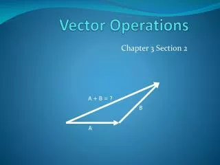
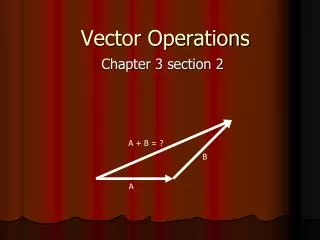
Repeated vector operationsa) divergence of the curl of a vector • The curl gives the magnitude and sense of the vector rotation confined within a prescribed region. • The divergence – monitors a vector field’s entry into or departure from a region (local source or sink within it). • Hence, a vector A with nonzero curl just rotates without entering or living the region
Repeated vector operationsb) the curl of a gradient of scalar function • The gradient of a scalar express the direction and magnitude that an inertialess ball would take as it rolls down a mountain along the path of least resistance. • The nonzero curl – requires that the ball will return to the top point • It is impossible without some new laws of nature like anti-gravitational forces
Repeated vector operationsc) gradient of a gradient of scalar function =>Laplacian • Def. Laplacian operation states that there is a vector field f where f is some scalar function • The divergence determines whether a source or sink exists at that point. • This operator is important for finding the potential distribution caused by charges. In mathematics and physics, the Laplace operator or Laplacian, named after Pierre-Simon de Laplace, is a differential operator, specifically an important case of an elliptic operator, with many applications. It is denoted by the symbols Δ,, or
Briefly about phasors • When sources in linear systems exhibit harmonic time dependence at a single fixed frequency • the corresponding phasor is as follows
Traveling wave • Phasors can be functions of positions such as: • What is adequate to the time-varying function
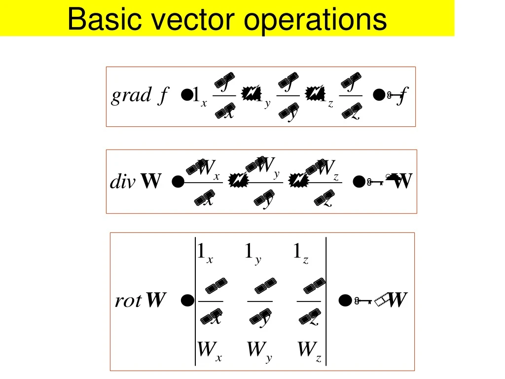
Vector identities are written in two forms: Using formal vector nabla and without it.
Gauss`s Theorem Theorem: Vector W flux through a closed surface S equals the volume integral of the vector W divergence over the volume bounded by S. This theorem enable us to change the volume integral of divergence over the volume V to the flux of the vector W through the boundary surface S. Conclusion: The flux of the sourceless field (div W=0 in each point of considered area) through the closed surface S equals zero.
Carl Friedrich Gauss 1777 - 1855 German mathematician and scientist
Problem: Calculate the flux of the vector W : through the sphere ofthe radius R=1 andwith the centre in the origin (0,0,0). Using Gauss’s theorem we calculate this flux as the volume integral of divergence field W.
Stokes’s theorem Theorem: Line integral of the vector W along the closed line c is equal to the flux of the vector rotation over the surface S bounded by the line c. This theorem enable us to change the surface integral of the rotation over the surface S to the line integral of the vector W along the boundary closed line c. Circulation of unrotational (irrotational) field (rot W=0 in each point of considered area) equals zero.
Sir George Gabriel Stokes, 1819 - 1903 Sir George Stokes communicated his theorem on the 1854.
Problem: Calculate the line integral of the vector W from previous problem along the circle with the radius R=2, laying in the xy plane, with centre in the point (0,0,0) For using Stokes’s theorem let’s calculate rotation of the field W:
z 1 1 y 5 x dS The flux of rot W is calculated through the disc laying on the plane xy, so vector dS is perpendicular to this plane, its direction is according to the z axis. Components rotxWand rotyW don’t generate the flux, because they are perpendicular to dS. Element ds represents the change of the integration surface (disc surface with the radius r) when its radius increases by dr.
Field potentials • Potential theory and theory of boundary problems are basic tools for solving field problems in mathematics. • Let’s introduce two of many potentials known in mathematics: • Scalar potential of the vector field W • Vector potential of the vector field W Scalar potential Let’s considerirrotational field W From vector calculus identity: Vector identity will be satisfied when
This is definition of scalar potential : If the scalar function φ exists we say that the field is potential. The necessary condition of field potentiality is its irrotationality. The surfaces which satisfy the equation are equipotential surfaces. We know, that vector W is always perpendicular to this surface.
Uniquenessof scalar potential From potential definition we conclude, that For the same vector W we can receive infinite number of potentials differing by a constant. Potential can be found unambiguously when we introduce the reference point in which potential equals zero. In practice it can be the set of points, i.e. the reference plane. Problem Potential of the vector field is given: 1.Calculate the constant C when φ=0 on yz plane 2. Calculate the components of the field W
hence 2. Solution 1. On the plane yz the variable x=0, so Let’s check whether this field is irrotational: All components of rotation are zero, the field is potential.
Problem Find scalar potential of the vector field W setting reference point N(1,1,1) Calculation of scalar potential We have to find the scalar function φ when vector components are known In considered area let’s agree that any point N(x0,y0,z0) will be treated as a reference point.
Solution Step 1 We integrate (1) with respect to x. The „constant” C1(y,z) appears in first iteration of solution φ(x,y,z) Step 2 We differentiate the potential received in step 1 i and compare it with (2).
C1 is independent on z, so is the constant number C1 is independent on y, so depends on z only. Step 3: We differentiate the potential received in step 2 and compare it with (3).
Step 4 We find constant C, if Received solution equals zero in set reference point. This procedure can be realized as fallows:
To minimize the number of symbols of the variables in integrated functions they are the same as integral limits.
Vector potential • Let’s consider vector field W in which: Definition of vector potential results from the vector identity
Let’s notice, that potential definition is ambiguous. From mathematical point of view we have many possibilities in determining of vector potential. This definition determines vector potential with precision to the gradient of any field, (to any potential field). To avoid this ambiguity we introduce an additional condition for field A. In practice it is the condition for divA.
The quantities describing electromagnetic field About history, briefly. • Ancient times-> 600 B.C. Thales of Miletus observed that rubbing of amber against a cloth caused the amber rod to attract light objects to itself • The use of amber had dramatic influence on the discipline that we now call electrical engineering and on the subject of electromagnetic fields. (amber=electron)
A new entity in nature that we call a charge was uncovered in those ancient experiments (fundamental as already encountered: mass, length, time) • Benjamin Franklin • Michael Faraday • Henry Cavendish • Charles-Augustin de Coulomb • Through a series of experiments, these scientists uncovered the fact that there would be a force of attraction for unlike charges and a force of repulsion for like charges.
Electric charge The feature of elementaryparticle which causes that the particles are subjects to electromagnetic operations. • Remark Charges of particles and systems of particles are elementary charge multiple:
Electric charge (cont.) 1C=1[Q] The charge unit is 1 Coulomb – it is the charge which is carried during 1 second through the given cross-section of the wire leading the DC current of 1 Amper. • Mass of the electron
Conclusions: • Electric charge of particles is not changing when particles are moving (does not depend on velocity) • The charge – means particular number of elementary particles. • Charge conservation law • Overall charge of isolated system is unchanging • Or • Algebraic sum of charges in the isolated system is constant.
First experiments in electricityCharles August Coulomb (F) 1736-1806 + + - WdWI 2015 PŁ
The very first measurement in electromagnetismCharles August Coulomb (F) 1736-1806 • On the basis of measurements Coulomb calculated the magnitude of the electric forces acting between charges • Torsion balance instrument
How? • A charges are inducted on a glass rod by rubbing it on a cloth and then touching it to two pith balls. • Changing the distance 2,3,4 times and the charge amount 2,4, 8 times • have found the formula (inverse aquare law): WdWI 2015 PŁ
Coulomb’s law Unit vector Distance between charges r WdWI 2015 PŁ
Coulomb’s law Point charges Permittivity of free space Coulomb’s force
Example 2.1 • Find the magnitude of the Coulomb force between an electron and a proton in a hydrogen atom. Compare with the gravitation force between these two particles, assume the distance between particles:
Example 2.1. Conclusion (ratio) It helps explain why chemical bonds that holds atoms, molecules, and compounds together can be so strong
In classic theory of electromagnetism we use several quantities which are right only in macro scale. I.e. the point charge can be considered only from outside. The point charge is the idealization of a real charge which can be gathered on unequal zero volume. We assumed that point charge volume tends to zero. The volume charge density – the ratio of the sum of the charges gathered in any area to its volume. The charge density describes a spatial distribution of the charge.
Analogically we can introduce the charge distributed on a surface or on a line. The surface charge density - the ratio of the sum of the charges gathered on any surface to its value. This density describes a surface distribution of the charge. The line charge density - the ratio of the sum of the charges gathered on any line to its length. This density describesa charge distribution along the line.
A point charge is the idealization of the real case, when a charge is gathered in an area which volume tends to zero. This notion „point charge” has the sense in macro scale only. The assumption, that the charge is gathered in point leads to the preposterous: the charge density tends to infinity. We can talk about point charge when we consider the electromagnetic field outside the charge.
The forces acting on the charge moving in electromagnetic field The Lorentz force The Lorentz force is the force acting on a point charge which is moving in electromagnetic field. It is given by the following equation in terms of the electric and magnetic fields. The electric and magnetic field are treated separately. This force can be used to define the basic field quantities: the intensity of electric field E and the induction of magnetic field B. If the electromagnetic field exists in linear medium, we can use for field describing the superposition method. In this method we separate both of the fields as two exciting quantities.
The physical quantities used in this formula: F is the force (in newtons – 1N) E is the electric field intensity (or simply electric field) (in volts per metre -1V/m ) B is the magnetic field induction (or simply magnetic field) (in teslas – 1T) q is the electric charge of the particle (in coulombs – 1C) v is the velocity of the particle (in metres per second – 1m/s) v×B is the vector product (has a sense of electric field) (in volts per metre 1V/m)
Beam of electrons moving in a circle, due to the presence of a magnetic field. Purple light is emitted along the electron path, due to the electrons colliding with gas molecules in the bulb.
Two forces: electric and magnetic will be used to define two vectors characterizing electric and magnetic fieldsacting alone. Definition of The electric field intensity (or simply electric field) is determined by following formula, when the charge is stationary.
The vector numerical value is given by: Vector direction is determined by such vector of charge velocity, where there is no force acting on the charge. Definition of For defining the vector we assume that only magnetic field exists, E=0. Because is the vector it has a length and a direction, hence its definition has2 parts.
We will introduce definition of current density which has two parts: for scalar J and for vector . Current conduction and current density. Free charges moving in the conducting medium form the electric current. This is dynamic phenomenon characterized by the vector of current density