LECTURE 11: EXPECTATION MAXIMIZATION (EM)
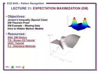
LECTURE 11: EXPECTATION MAXIMIZATION (EM). Objectives: Jensen’s Inequality (Special Case) EM Theorem Proof EM Example – Missing Data Intro to Hidden Markov Models Resources: Wiki: EM History T.D.: Brown CS Tutorial UIUC: Tutorial F.J.: Statistical Methods. Audio:. URL:. Synopsis.

LECTURE 11: EXPECTATION MAXIMIZATION (EM)
E N D
Presentation Transcript
LECTURE 11: EXPECTATION MAXIMIZATION (EM) • Objectives:Jensen’s Inequality (Special Case)EM Theorem ProofEM Example – Missing DataIntro to Hidden Markov Models • Resources:Wiki: EM HistoryT.D.: Brown CS TutorialUIUC: TutorialF.J.: Statistical Methods Audio: URL:
Synopsis • Expectation maximization (EM) is an approach that is used in many ways to find maximum likelihood estimates of parameters in probabilistic models. • EM is an iterative optimization method to estimate some unknown parameters given measurement data. Used in a variety of contexts to estimate missing data or discover hidden variables. • The intuition behind EM is an old one: alternate between estimating the unknowns and the hidden variables. This idea has been around for a long time. However, in 1977, Dempster, et al., proved convergence and explained the relationship to maximum likelihood estimation. • EM alternates between performing an expectation (E) step, which computes an expectation of the likelihood by including the latent variables as if they were observed, and a maximization (M) step, which computes the maximum likelihood estimates of the parameters by maximizing the expected likelihood found on the E step. The parameters found on the M step are then used to begin another E step, and the process is repeated. • This approach is the cornerstone of important algorithms such as hidden Markov modeling and discriminative training, and has been applied to fields including human language technology and image processing.
Special Case of Jensen’s Inequality • Lemma: If p(x) and q(x) are two discrete probability distributions, then: • with equality if and only if p(x) = q(x) for all x. • Proof: • The last step follows using a bound for the natural logarithm: .
Special Case of Jensen’s Inequality Continuing in efforts to simplify: We note that since both of these functions are probability distributions, they must sum to 1.0. Therefore, the inequality holds. The general form of Jensen’s inequality relates a convex function of an integral to the integral of the convex function and is used extensively in information theory.
The EM Theorem Theorem: If then . Proof: Let y denote observable data. Let be the probability distribution of y under some model whose parameters are denoted by .Let be the corresponding distribution under a different setting .Our goal is to prove that y is more likely under than .Let t denote some hidden, or latent, parameters that are governed by the values of . Because is a probability distribution that sums to 1, we can write: Because we can exploit the dependence of y on t and using well-known properties of a conditional probability distribution.
Proof Of The EM Theorem We can multiple each term by “1”: where the inequality follows from our lemma. Explanation: What exactly have we shown? If the last quantity is greater than zero, then the new model will be better than the old model. This suggests a strategy for finding the new parameters, – choose them to make the last quantity positive!
Discussion • If we start with the parameter setting , and find a parameter setting for which our inequality holds, then the observed data, y, will be more probable under than . • The name Expectation Maximization comes about because we take the expectation of with respect to the old distribution and then maximize the expectation as a function of the argument . • Critical to the success of the algorithm is the choice of the proper intermediate variable, t, that will allow finding the maximum of the expectation of . • Perhaps the most prominent use of the EM algorithm in pattern recognition is to derive the Baum-Welch reestimation equations for a hidden Markov model. • Many other reestimation algorithms have been derived using this approach.
Example: Estimating Missing Data • Consider a data set with a missing element: • Let us estimate the value of the missing point assuming a Gaussian model with a diagonal covariance and arbitrary means: • Expectation step: • Assuming normal distributions as initial conditions, this can be simplified to:
Example: Gaussian Mixtures • An excellent tutorial on Gaussian mixture estimation can be found at J. Bilmes, EM Estimation • An interactive demo showing convergence of the estimate can be found atI. Dinov, Demonstration
Summary • Introduced a special case of Jensen’s inequality. • Introduced and derived the Expectation Maximization Theorem. • Explained how this can be used to reestimate parameters in a pattern recognition system. • Worked through an example of the application of EM to parameter estimation. • Introduced the concept of a hidden Markov model.