Dynamic Treatment Regimes: Sequential, Multiple Assignment Randomized Trials in Survival Analysis
This paper presents insights into dynamic treatment regimes structured as sequential, multiple assignment randomized trials (SMART) designed for effective survival analysis. By adapting treatment types and dosages based on patient responses, SMART trials allow for tailored interventions to optimize outcomes. We explore the principles behind SMART designs, including decision rules and methodologies used in various treatment applications, such as ADHD and alcoholism. Additionally, we discuss weighted test statistics and sample size determination to refine analysis in complex clinical landscapes.

Dynamic Treatment Regimes: Sequential, Multiple Assignment Randomized Trials in Survival Analysis
E N D
Presentation Transcript
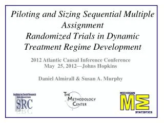
Sizing Sequential, Multiple Assignment, Randomized Trials for Survival Analysis Z. Li & S.A. Murphy In Honor of Tom Ten Have April, 2012
Tom Attributes Self -effacing Always Encouraging Helps others Upbeat Idea generator Asks hard questions Role model
Dynamic treatment regimes are individually tailored treatments, with treatment type and dosage changing according to patient outcomes. Conceptualize treatment as a series of stages. 2 Stages for one individual Observation available at jth stage Action at jth stage (usually a treatment)
A dynamic treatment regime is the sequence of two decision rules: d1(X1), d2(X1,d1,X2) for selecting the actions in future. In many survival analysis trials, the observation X2 includes an indicator of response/non-response and whether the failure time has occurred.
Our Goal is to design a sequential, multiple assignment, randomized trial (SMART). These are trials in which subjects are randomized among alternative options (the Aj’s are randomized) at each stage. Example of a simple regime: No X1, d1= 1 (tx coded 1) X2 = R, an indicator of early signs of non-response, d2(1,R) = 0 if R=1 (tx coded 0) otherwise stay on current tx
SMART • Precursors of the SMART design: • CATIE (2001), STAR*D (2003), many in cancer • SMART designs: • Treatment of Alcohol Dependence (Oslin, data analysis; NIAAA) • Treatment of ADHD (Pelham, data analysis; IES) • Treatment of Drug Abusing Pregnant Women (Jones, in field; NIDA) • Treatment of Autism (Kasari, in field; Foundation) • Treatment of Alcoholism (McKay, in field; NIAAA) • Treatment of Prostate Cancer (Millikan, 2007)
ADHD (Pelham, PI) Continue, reassess monthly; randomize if deteriorate Yes 8 weeks A1=1. Begin low-intensity BEMOD A2=1 Add medication;BEMOD remains stable Assess- Adequate response? Randomassignment: No A2=0 Increase intensity of BEMOD Randomassignment: Continue, reassess monthly; randomize if deteriorate 8 weeks A2=0 Increase dose of medication A1=0.Begin low dose medication Assess- Adequate response? Randomassignment: A2=1 Add BEMOD,medication dose remains stable No
Background Survival probabilities (and associated tests) Lunceford et al. (2002) 3 weighted sample proportion estimators Wahed and Tsiatis (2006) semiparametric efficient + implementable estimator Miyahara and Wahed (2009) weighted Kaplan-Meier estimator. Feng and Wahed (2009) sample size formulae based on a Lunceford et al. estimator Guo and Tsiatis (2005) weighted cumulative hazard estimator Weighted version of the log rank test Guo(2005) proposes weighted log rank test Feng and Wahed (2008) weighted version of supremum log rank test and associated sample size formulae
Notation • Suppose we decide to size the study to compare regimes (A1, A2)= (1,1) versus (A1, A2)= (0,1) • Randomization probabilities are p1, p2 • T11, T01potential failure times under each regime • T, S, C are the failure time, time to nonresponse, censoring time, respectively • R is the nonresponse indicator, e.g. R=1S≤min(T,C)
Test Statistics • Weighted version of the Kaplan-Meier to test • Weighted version of the log rank test to test Selected time point (usually end of study) Survival function
Weights Weights are necessary to adjust for the trial design. • Time independent weights (for regimes 11 and 01): • Time dependent weights (potentially more efficient): R=1S≤min(T,C)
Weighted Kaplan-Meier (WKM) Estimator • Time dependent weights (tWKM): -Asymptotically normal with mean and variance • Can use the time independent weights (cWKM) as well. (j,k)=(1,1), (0,1) ith subject,
Weighted Log Rank Test (WLR) Time dependent weights (tWLR): where (j,k)=(1,1), (0,1) and Asymptotically normal under a local alternative, PH assumption, with mean, and variance Can use the time independent weights (cWLR) as well.
Sample Size Formulae • Test based on WKM estimator: • WLR test:
Challenges • Variances are complex and depend on the joint distribution of the failure time T and the time to non-response, S. • These two times are likely dependent. • It may be hard to elicit information about this joint distribution in order to design the trial.
Our Approach • Use time independent weights in the sample size formulae (cWKM or cWLR). • Express the variances in terms of the potential failure times under each regime, Tjk, e.g. in terms of • Replace variances with simpler upper bounds.
The Variances via Potential Outcomes • cWKM: • cWLR:
Upper Bounds on Variances (Replace R by 1)
Sample Size Formulae • Test based on cWKM: where • cWLR:
Data Analysis Use potentially more powerful tests than that used for sample size calculation. Testing • Test based on tWKM • Test based on Lunceford 3 (Lunceford et al, 2002) • Test based on Wahed and Tsiatis, (2006) implementable estimator, WT Testing • tWLR
Simulation • Proportional hazards for T11and T01 • Frank Copula model for potential outcomes (Tjk, Sj) to produce a positive dependency • Weibull marginal distributions for Tjk and Sj • Compare with Feng and Wahed (2009) sample size formula: • Based on a weighted sample proportion estimator (the second estimator in Lunceford et al., 2002). • Assumed independence between Tjk and Sj to simplify variances.
Discussion • Working assumptions used to size the study are the same as the working assumptions used to size a standard two arm study. • Sample sizes are conservative; the degree of conservatism depends on the percentage of subjects with R=1. • cWLR yields smaller sample sizes than cWKM and needs less information, but power guarantees rely on proportional hazards assumption. • These formulae can be easily generalized to more complex designs with the number of treatment options differing by both response status and prior treatment.
This seminar can be found at: http://www.stat.lsa.umich.edu/~samurphy/ seminars/ENAR.04.2012.ppt Email Zhiguo Li or me with questions or if you would like a copy: zhiguo.li@duke.edu or samurphy@umich.edu
Timing of movement between stages The timing of the stages may be fixed or may be an outcome of treatment. -----suppose the second stage is only for non-responders Fixed timing: Second stage starts at 8 weeks after entry into trial. Random timing: Second stage starts as soon as a nonresponse criterion is met.