Binary Choice Models
Binary Choice Models. Topic Overview. Introduction to binary choice models The Linear Probability model (LPM) The Probit model The Logit model . Introduction. In some cases the outcome of interest ( Y ) is not quantitative, but a binary decision: Go to college or not

Binary Choice Models
E N D
Presentation Transcript
Topic Overview • Introduction to binary choice models • The Linear Probability model (LPM) • The Probit model • The Logit model
Introduction • In some cases the outcome of interest (Y) is not quantitative, but a binary decision: • Go to college or not • Adopt a technology or not • Join the union or not • For example, how well do an individual’s socioeconomic characteristics explain his/her decision to join a trade union? • Often such models are used to model decisions: to invest or not, to enter a market or not, to hire or not, to adopt a technology or not… • Binary variables as dependent variables (Y) complicate the estimation process
Introduction • Only suitable where we can plausibly narrow down the decision alternatives to two. • Qualitative models where the choice is between two discrete, mutually exclusive and jointly exhaustive alternatives. • Y, the dependent variable is these models is binary or dichotomous; it can only takes on the values of 0 or 1. • Also known as ‘rational choice’ models – as Y often represents a rational choice between two alternatives. The Xs are the factors that are expected to contribute to the selection of one outcome over another.
An Example • The decisions of farmers to adopt to the latest technology: Yi= β1+ β2 Xi +...+ ui • where Yiis a binary variable, representing two choices, e.g. to adopt (Y=1) the latest technology or not to adopt (Y=0) • The decision is influenced by economic , structural, farm and farmer characteristics • For example costs, farm size, age of the farmer, access to credit etc. • So, we might for instance find that age of the farmer negatively affects the probabilityof adoption, while farm size has a positive effect
Alternative Models • There are several ways to estimate a binary choice model: • The Linear Probability Model (LPM) • The Probit Model • The Logit Model
The Linear Probability Model • Linear regression model with binary dependent variable Yi = 1+ 2Xi + 3Xi +…+ ui • The conditional expectations E(Yi|Xi) can be interpreted as the conditionalprobability that the event (Yi) will occur given Xi: E(Y|X1, X2,…,Xk) = P(Y=1|X1, X2,…,Xk) • E(Yi|Xi) might express the probability of purchasing a durable good (e.g. a car) for a given level of Xi (e.g. income). • Estimated with OLS
The Linear Probability Model • The conditional expectation of the model can be interpreted as the conditional probability of Yi, or: E(Yi|Xi) = β1 + β2 Xi = Pi [ui is omitted since we have assumed that E(ui)=0 ] • Pi = probability thatYi = 1 and (1-Pi) = probability Yi =0 • Yi follows what is known as the Bernoulli probability distribution: • The fact thatYiis a probabilistic term imposes a very important restriction in the values it can take: 0 ≤ E(Yi|Xi) ≤ 1
An Example of the LPM • Estimate the determinants of trade union membership (variable union) • normal OLS regression with union as our dependent variable; • In Stata: regress union exp sex
Stata Output and Interpretation • The above can be interpreted as follows: • “the slope coefficient measures the change in the average value of the regressand for a unit change in the value of a regressor, with all other variables held constant” • In this case, holding other variables constant, an increase by one unit in exp (on-the-job experience) increases the probability of union membership by 0.004
Problems: LPM • Simple model but there are important shortcomings: • Non-normality of the disturbances • Heteroskedasticity • Nonsense probabilities • Implausibility of linearity
Non-normality of the disturbances • In the LPM the disturbances ui are: ui = Yi - β1 - β2 Xi • Just like Yi, ui also takes only two values. • This makes the assumption of normality in the distribution of ui(necessary for inference) unattainable. • In fact the probability distribution of ui in the LPM is: • Possible to overcome by central limit theorem
Heteroscedasticity • The (binomial) Bernoulli probability distribution implies by definition a non-constant variance • Specifically the variance would be: var(ui)= Pi(1-Pi) • Since the expected probability of an event happening varies for each case, then we can no longer assume a constant variance Pi= E(Yi|Xi) = β1 + β2 Xi • Usual remedial measures may be employed to correct for heteroscedasticity(e.g. WLS)
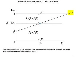
Nonsense Probabilities • Due to its probabilistic nature: 0 ≤ Yi≤ 1 • In practice though, OLS estimates of Yi may be more than 1 or less than 0. • We can still ‘constrain’ those estimates to the desired boundaries, but the adjustment is not very good. If some of the estimated Ŷs are less than 0 (that is, negative), Ŷiis assumed to be zero for those cases; if they are greater than 1, they are assumed to be 1.
Implausible Linearity • The LPM assumes a linear relationship between the levels of the X variable(s) and the probability that Y=1. • This linearity (or constant effect of X on Y) is very implausible. • Consider the case of a family’s decision to own a house – would the probability be the same for all levels of income? • It is more plausible to expect that the probability is progressively higher or lower for different levels of income… • All this indicates that the LPM is probably not a very good model. • Probit and logit models offer significant advantages and should be preferred
Probit and Logit Models • Alternative models that are less problematic are the probit and the logit model • The relationship between Piand Xi is non-linear • AsXiincreases, the conditional probability of an event occurring Pr(Yi=1|Xi) increases but never steps outside the 0-1 interval • Due to this built-in non-linearity both use an alternative estimator to OLS; the Maximum-Likelihood (ML) method
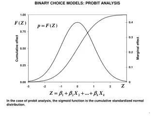
Probit and Logit Models • Cumulative distribution function (s-shaped). • Normal distribution – probitor logistic distribution – logit. • Unlike the linear probability model the predicted probabilities are between 0 and 1.
The Probit Model • The probit model can be derived from an underlying latent variable model that satisfies the classical linear assumptions • The outcome decision depends on an unobservable utility index: Ii= β1 +β2 Xi + ui • For example, decision Y to own a house (Y=1) or not (Y=0) depends on an unobservable utility index Ii, that is determined byXi(e.g. income, number of children) • The larger the value of Ii the greater the probability of Y =1 (e.g. owning a house)
The Probit Model • The latent (unoberservable) variable Iiis linked to the observed decision Yiby: • If a person’s utility indexIexceeds the threshold level I* (here assumed to be 0) Y=1, and if not, then Y=0 • It is assumed that the error term u is independent of X and follows a standard normal distribution • The error is symmetrically distributed about 0, which means that 1-F(-z) = F(z)
The Probit Model • Hence the normal distribution allows us to compute the probability that Y=1 • With F being the standard normal cumulative distribution function (CDF) • This ensures that the probability is strictly between 0 and 1
The Normal CDF • That is, in the probit model, Pi the conditional probability that Yi=1 (given Xi), follows the normal CDF. • So if we plot the probabilities that Yi=1 for different (given) X values cumulatively we get: Pi Xi -∞ + ∞ 0
Interpreting the Results: Probit • Interpreting the slope coefficients of the probit model is complicated • Marginal effects: where is the probability density function of the standard normal variable and Zi = β1 +β2 Xi +...+ βk Xi • The sign of the marginal effect is the same as βi • The magnitude of the change depends on the magnitude ofβiand the value Zi • All X variables are involved in computing the changes in probability • Marginal effects vary for different levels of X; it is customary to estimate them at the mean of the variables.
Interpreting the Results: Probit …it follows that the marginal effects of X on Y, vary for different levels of X Low marginal effects at extreme values of X, high marginal effects at central values. Pi Xi -∞ + ∞ 0
Stata Output .0064 x (-1.12cons+0.006exp+(-.54sex)+(-.33sth)+.01age)
Interpreting the Results: Probit • If X2 is a binary variable the marginal effect from changing from 0 to 1 is • Again, this depends on all values of the other explanatory variables
The Logit Model • The logit model is similar to the probit model – the key difference is that it is based on the logistic CDF rather than the normal CDF. • If the utility index exceeds the threshold level I*, Y=1, otherwise Y=0 • Assuming F to be a logistic CDF • Where
Pi 1 Xi - ∞ 0 + ∞ The Logistic CDF
Interpreting the Results: Logit • The ratio of the two probabilities is the odds ratio in favor of the outcome: • The logit model produces easily communicable odd ratios of the marginal effects of a single unit’s increase in each independent variable on the probability of Y=1. • The ratio P/(1-P) is the odds ratio in favour of owning a house – ratio of the probability that a family will own a house to the probability that it will not own a house
Interpreting the Results: Logit • Marginal effects can be calculated in the same way as for the probit model • Also possible to calculate the odds ratios • odds ratio = eβ • where e (the natural logarithm) equals approximately 2.71828 • If eβ is greater than 1, the odds are eβ times larger • If eβ is less than 1, the odds are eβ times smaller • Positive effects are greater than 1, while negative effects are between 0 and 1
Stata Output eβ 2.71828 -9625674= 0.3819 “holding other regressors constant, women (sex=1) are approximately 3.8 times less likely to be a member of union”
Estimation: Probit and Logit • Estimation using OLS is not possible due to non-linearity not only in the variables but also in the parameters (the betas). • Maximum Likelihood is the suitable method: it involves maximising a likelihood function in such a way that the resulting betas take those values that maximise the probability of observing the given Y’s. • For the precise mechanics (see GUJ Appendix 15A.p. 633). • In practice software (in our case Stata) does all the hard work for us: • Command Syntax in stata: probit /logit <Y variable> <X variables> • e.g. probit union exp sex
Inference: Probit and Logit • Likelihood ratio (LR) statistic: • Tests the null hypothesis that all β coefficients are zero (equivalent to the F-test in the linear regression model). • The LR statistics follows the chi-square distribution (χ2) with df equal to the number of explanatory variables (constant not included), e.g. LR chi2(3) = 27.55 • Wald-statistic • Tests the null hypothesis that β=0 (equivalent to t-statistic) • inferences are based on the normal table (if sample is large, t-distribution converges to the normal distribution) • Stata provides exact p values that the null hypothesis is true for both tests.
Goodness of Fit: Probit and Logit • Conventional R2 is not very meaningful in probit or logit models. • Many alternative measures have been proposed, the most widely used are the Count R2 and McFadden R2. • Count R2: • McFadden R2 (Pseudo R2): Calculated as • Expected signs and significance of coefficients is important
Example in Stata After estimating either a probit or a logit, type fitstat to obtain Goodness-of-Fit statistics:
Probit or Logit? • Respective CDFs are almost identical:
Probit and Logit • The two models can be used interchangeably: there are no good theoretical reasons to prefer one over the other. • Their results should be qualitatively identical; i.e. we should get the same coefficient signs regardless of whether we use probit or logit. • “ … if you multiply the probit coefficient by about 1.81 (which is approximately = π/√3), you will get approximately the logit coefficient (…) Alternatively, if you multiply a logit coefficient by 0.55 (= 1/1.81), you will get the probit coefficient” • Sometimes the logit is preferred due to the easy interpretation of its coefficients through odds ratios • Sometimes the probit is preferred due to its normal distribution assumption • You can begin by running a logit, perform the tests and to test for robustness also try a probit – then compare the output.