Download
1 / 75
790 likes | 1.27k Vues
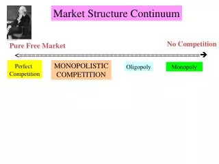
Chapter 11 – Market Structure: Perfect Competition, Monopoly, and Monopolistic Competition. Perfect Competition and Monopoly: Extremes. Market structures can be represented, in terms of a firm’s market power, as a continuum: Price Takers Price Searchers. Imperfect Compeition.

E N D
Chapter 11 – Market Structure: Perfect Competition, Monopoly, and Monopolistic Competition
Perfect Competition and Monopoly: Extremes • Market structures can be represented, in terms of a firm’s market power, as a continuum: • Price Takers Price Searchers Imperfect Compeition Perfect Competition Monopoly Zero Market Power Maximum Market Power
Two Broad Categories of Market Types • Price Takers Markets • Perfect competition • Price Searchers Markets • Monopoly • Monopolistic competition • Oligopoly
Price Takers • Price Takers produce identical products and each seller is small relative to the market. • Each seller has little or no effect on the market price. • Each firm can sell as much as it wantsat the market price • It is unable to sell any output at a price greater than the market price Example: agriculture(wheat, corn, soybeans) Also called purely competitive market or perfect competition.
Price Searchers • Price Searchers face a downward sloping demand curve for their product. • The amount that the firm is able to sell is inversely related to the price it charges. • Examples: • Nike, • General Motors, • Exxon, • most retail stores
2. Markets When Firms are Price Takers (Perfectly Competitive Firms)
Conditions for a Market of Price Takers • All firms produce an identical product. • A large number of firms are in the market. • Each firm supplies only a small portion of the total supplied to the market. • No barriers to entry or exit exist.
Price is determinedin the market. Price Price MarketSupply Individual firms musttake the market price. P P Demand forSingle Firm MarketDemand Output / Time Output / Time Price Taker’s Demand Curve • The market forces of supply and demand determine price. • Price takers have no control over the price that they may charge in the market. If such a firm was to offer their good/service at a price above that established by the market, then consumers would simply buy elsewhere. • Thus, the demand for the product of the firm is perfectly elastic. Only at the market price will there be any demand.
3. Output in the Short Run in Price Takers’ (Perfectly Competitive) Markets
MarginalRevenue (MR) = the change in total revenue the change in output Marginal Revenue • Marginal Revenue is the change in total revenue divided by the change in output. • In a price taker market, Marginal Revenue = Market Price.
MC p = MC Profit ATC P d(P = MR) C A P > MC P < MC decrease q Increase q Profit Maximization when the Firm is a Price Taker • In the short run, the price taker will expand output until marginal revenue (price) is just equal to marginal cost. Price • This will maximize the firm’s profits (rectangle BACP). B • When P > MCthen the firm can make more on the next unit sold than it costs to increase output for that unit. In order for the firm to maximize its profits it increases output until MC= P. • When P < MCthen the firm made less on the last unit sold than it cost for that unit. In order for the firm to maximize its profits it decreases output until MC= P. Output/ Time q 0
TotalRevenue(TR) Profit(TR - TC) TotalCost(TC) Output 0 1 2 . . . . . . . 8 9 Profits occurwhereTR > TC 10 TC 11 Profits Maximizedwhere difference is largest TR 12 13 14 15 16 17 Losses occurwhereTC > TR 18 19 20 21 Total Revenue / Total Cost Approach • An alternative way of viewing profit maximization within the firm focuses on the relationship between total revenue (TR) and total cost (TC). 0 25.00 - 25.00 • At low levels of output profits are negative as total costs exceed total revenue. 5 29.80 - 24.80 10 33.75 - 23.75 • After some point, total revenues may exceed total costs. Profit is maximized where this difference is maximized. . . . . . 48.00 - 8.00 40 - 4.25 45 49.25 Average and/or Marginal Product - .25 50 50.25 125 55 3.50 51.50 6.75 60 53.25 100 9.25 65 55.75 10.75 70 59.25 75 11.00 75 64.00 10.00 80 70.00 50 85 77.25 7.75 4.50 90 85.50 0.00 25 95 95.00 - 8.00 100 108.00 Output Level - 20.00 125.00 105 2 4 8 10 6 16 12 14 20 18 22
MarginalRevenue(MR) Profit(TR - TC) MarginalCost(MC) Output 0 1 2 . . . . . . . 8 MC 9 10 11 Profit MaximumP = MR = MC 12 13 14 15 16 17 18 19 20 21 Marginal Revenue / Marginal Cost Approach • We can show the relationship between theTR/TC and the MR/MC approach. • Below, low levels of output delivermarginal revenue to the firm greater than the marginal cost of increased output. ---- ---- - 25.00 5 $ 4.80 - 24.80 • After some point, though, additional units cost more than their marginal revenue. 5 $ 3.95 - 23.75 . • Profit is maximized where P= MR = MC. . . . . • Both the TR/TC and the MR/MC method yield the same profit maximizing output, q=15 $ 1.50 - 8.00 5 - 4.25 5 $ 1.25 Price and CostPer Unit - .25 5 $ 1.00 9 5 3.50 $ 1.25 6.75 5 $ 1.75 7 9.25 5 $ 2.50 MR 10.75 5 $ 3.50 5 11.00 5 $ 4.75 10.00 5 $ 6.00 3 5 $ 7.25 7.75 4.50 5 $ 8.25 0.00 1 5 $ 9.50 - 8.00 5 $ 13.00 Output Level - 20.00 $ 17.00 5 2 4 8 10 6 16 12 14 20 18 22
MC ATC Loss AVC A d(P = MR) C P2 P1 p = MC Operating with Short-Run Losses • In the graph to the right, the firm operates at an output level where p = MC, but here ATC > MC resulting in a loss for the firm. Price • The magnitude of the firm’s short-run losses is equal to the size of the of the rectangle BACP1 • A firm experiencing losses but covering its average variable costs will operate in the short-run. B • A firm will shutdown in the short-run whenever price falls below average variable cost (P2). • A firm will shutdown in the long-run whenever price falls below average total cost. Output/ Time q 0
Firm’s Short-Run Supply Curve • A firm maximizes profits when it produces at P=MC and variable costs are covered - this is the GOLDEN RULE of profit-maximization. • A firm’s short-run supply curve is its marginal cost curve above average variable cost.
Short-Run Market Supply • The short-run market supply is the horizontal sum of the all firms’ short-run marginal cost curves
Price Price MC is thefirm’ssupply curve MC Ssr(MC) ATC AVC Output Output Representative Firm Market Supply Curve for the Firm and the Market • Given resource prices, the marginal cost curve (MC) is the representative firm’s supply curve for a specific good. • As price rises above the short-run shutdown price of P1,, the firm will supply additional units of the good. • The short-run market supply curve (Ssr) is merely the sum of the MCs of all the firms. • Note that below P1 no quantity is supplied because P < AVC. P3 P3 P2 P2 P1 P1 q1 q2 q3 Q1 Q2 Q3
1. How do firms that are price takers differ from those that are price searchers? What are the distinguishing characteristics of a price taker market? Questions for Thought: 2.Why is competition in a market important? Is there a positive or negative impact on the economy when strong competitive pressures drive various firms out of business? Why or why not?
4. Output Adjustments in the Long Run in Price Takers’ (Perfectly Competitive) Markets
Economic Profits and Entry • If price exceeds average total cost, firms will earn an economic profit. • Economic profit induces both • entry of new firms • expansion in the scale of operation of existing firms. • Capital moves into the industry, shifting the market supply to the right. This will continue until price falls to ATC • In the long-run, competition drives economic profit to zero.
Economic Losses and Exit • If average total cost exceeds price, firms will suffer an economic loss. • Economic losses induce • exit of firms from the market • a reduction in the scale of operation of remaining firms. • As market supply decreases, price will rise to average total cost. • Thus, profits and losses move price toward the zero-profit long-run equilibrium.
Ssr Price Price MC ATC P1 d D Output Output Firm Market Long-run Equilibrium • The two conditions necessary for long-run equilibrium in a price-taker market are depicted here. • First, the quantity supplied and the quantity demanded must be equal in the market, as shown below at P1 with output Q1. • Second, the firms in the industry must earn zero economic profit (that is, the “normal market rate of return”) at the established market price (P1 below). P1 q1 Q1
S1 S2 Price Price MC ATC P2 P1 d2 d1 D2 D1 Output Output Firm Market Adjusting to Expansion in Demand • Consider the market for toothpicks. If the introduction of a new candy product that sticks to one’s teeth causes the market demand for toothpicks to increase from D1 to D2 . . . • . . . the market price for toothpicks rises to P2 . . . • . . . shifting the firm’s demand curve upward. At the higher price, firms will expand output to q2 and earn short-run profits. • The economic profits will draw competitors into the industry, shifting the market supply curve from S1 to S2. P2 P1 q1 q2 Q1 Q2
S2 Price Price MC ATC Slr P1 P2 P1 d1 d2 d1 D1 D2 Output Output Firm Market Adjusting to Expansion in Demand • After the increase in market supply, a new equilibrium is established at the original market price (P1) and a larger rate of output (Q3). • As the market price returns to P1, the demand curve facing the firm returns to its original level. • In the long-run, economic profits are driven down to zero. • Note the long-run market supply curve is flat (Slr). S1 P2 P1 P1 q1 q1 q2 Q1 Q2 Q3
S1 S2 Price Price MC ATC P2 P1 d2 d1 D2 D1 Output Output Firm Market Adjusting to a Decline in Demand • If, instead, something occurs that causes market demand for toothpicks to decrease from D1 to D2 . . . • . . . the market price for toothpicks falls to P2 . . . • . . . shifting the firm’s demand curve downward, inducing a reduction in output to q2. The firm is now making losses. • Short-run losses cause some competitors to go out of business, and others to reduce the scale of their operation, shifting the market supply curve from S1 to S2. P1 P2 q2 q1 Q2 Q1
S2 Price Price MC ATC Slr P1 P2 P1 d2 d1 d1 D2 D1 Output Output Firm Market Adjusting to Decline in Demand • After the decrease in market supply, a new equilibrium is established at the original market price (P1) and a smaller rate of output (Q3). • As the market price returns to P1, the demand curve facing the firm returns to its original level. • In the long-run, economic profit returns to zero. • Note the long-run market supply curve is flat (Slr). S1 P1 P1 P2 q2 q1 q1 Q3 Q2 Q1
Long Run Supply • Constant-Cost Industry: Industry where per-unit costs remain unchanged as marketoutput is expanded. • Occurs when the industry’s demand for resource inputs is small relative to the total demand for the resources. • The long-run market supply curve in a constant-cost industry is horizontal.
Long Run Supply • Increasing-Cost Industry: Industry where per-unit cost rises as market output is expanded. • Results because an increase in industry output generally leads to stronger demand and higher prices for the inputs. • The long-run market supply curve in a increasing-cost industry is upward-sloping. • Most common type of industry
Long Run Supply • Decreasing-Cost Industry: Industry were per-unit costs decline as market output expands. • Implies either economies of scale exist in the industry or that an increase in demand for inputs leads to lower input prices. • The long-run market supply curve in a decreasing-cost industry is downward-sloping. • Decreasing-cost industries are uncommon.
Price Price S2 S1 MC2 MC1 ATC2 ATC1 P1 d1 P1 D2 D1 q1 Q1 Output Output Firm Market Increasing Costs and Long-Run Supply • Consider the market below, where an increase in the market demand pushes up the market price, leading to short-run profits for the individual firms. • Economic profit entices some new firms to enter the market and others to increase the scale of their operation. . . • . . . shifting out the market supply curve and lowering the market price. The firm’s costs are now higher (ATC2 & MC2) because the stronger demand for inputs pushes their price up. P2 Q2
Price Price Slr MC2 ATC2 P3 P1 d2 d1 D1 D2 Output Output Firm Market Increasing Costs and Long-Run Supply • This process continues until economic profits are eliminated. • At the new equilibrium price (P3), a larger quantity is supplied to the market (Q3). • Because this is an increasing-cost industry, expansion in market output leads to a higher equilibrium price. • Thus, the long-run supply curve (Slr) is upward sloping. S2 S1 MC1 ATC1 P2 P3 P1 q1 Q1 Q3 Q2
Price determination in PC markets Supply P = 22 - .5Qd P = 4 + .25Qs Price $10 Demand Quantity 24
Using calculus P = PQ - TC dP/dQ = P -dTC/dQ = 0 at the optimum. ==> P = MC d2TC/dQ2 > 0 ==> marginal costs rising
THE FIRM UNDER PERFECT COMPETITION • EFFICIENCY AND THE PERFECTLY COMPETITIVE MODEL • PRODUCTIVE EFFICIENCY: Under PC, firms are forced to minimize ATC and to charge prices such that P=minimum ATC • ALLOCATIVE EFFICIENCY: Under PC, the profit maximization rule P=MC assures the most efficient allocation of resources in the production of goods and services most desired by consumers
THE FIRM UNDER PERFECT COMPETITION • LIMITATIONS OF THE PERFECT COMPETITION MODEL: • Ignores real-world economies of scale • Ignores real-life variety of demands and variety of products supplied • Does not depict real-life dynamic behavior and disequilibrium situations • Focuses on price competition rather than multi-dimensional real-life competition
3. Markets Where Firms Are Price Searchers With High Entry Barriers:The Case of Monopoly
Monopoly • Monopoly is a market with: • High entry barriers • Single seller of a well-defined product for which there are no good substitutes. • Only a few markets exist with a single seller but it is worth studying. • Help us understand markets with few sellers.
Entry Barriers • Economies of Scale • Government Licensing • Patents • Control Over an Essential Resource
Price and Output Under Monopoly • The market demand curve is the monopolist’s demand curve • Monopolists will expand output until marginal revenue equals marginal cost. • The monopolist will charge the price on the demand curve consistent with that output.
Reduction inTotal Revenue Increase inTotal Revenue Marginal Revenue of a Price Searcher • Consider a market for a product where the initial price is P1 and output q1. Total revenue = P1 * q1. Price • When a firm faces a downward sloping demand curve, a price reduction that increases sales will exert two conflicting influences on total revenue. • As we decrease price from P1 to P2, output increases from q1 to q2. What effects does this have on total revenue? P1 P2 • First, total revenue will rise because of an increase in the number of units sold (q2 - q1) * P2. d • However, total revenue will decline by [(P1 - P2) * q1] because q1 units that were previously sold at the higher price (P1) are now sold at the lower price (P2). MR • Depending on the size of the respective shaded regions, total revenue may increase or decrease. q2 q1 Quantity /Time
EconomicProfits A B MR< MC MR> MC decrease q Increase q Price and Output Under Monopoly Price MC • A monopolist will reduce price and expand output as long as MR >MC • A monopolist will increase price and shrink output when ever MR <MC ATC P • Output level q will result . . . . . . with price P. C • At q the average total cost is C . . . d • As P > C (price > ATC) the firm is making economic profits equal to the shaded area, ( APCB). MR q Quantity / Time .
TotalRevenue(1)*(2)(3) TotalCosts(Per Day)(4) Profit(3) - (4)(5) MarginalCost(6) MarginalRevenue(7) Rate of Output(Per Day)(1) Price(Per Unit) (2) -$50.00 $50.00 0 ---- ---- ---- ----- $60.00 $25.00 $25.00 -$35.00 $10.00 $25.00 1 2 $69.00 $48.00 $24.00 -$21.00 $9.00 $23.00 3 $77.00 $69.00 $23.00 -$8.00 $8.00 $21.00 $84.00 $88.00 $22.00 4 $4.00 $7.00 $19.00 $90.50 $105.00 5 $21.00 $14.50 $6.50 $17.00 $96.75 $118.50 $19.75 $21.75 $6.25 $13.50 6 $102.75 $129.50 $18.50 $26.75 $6.00 $11.00 7 $108.50 8 $138.00 $17.25 $29.50 $5.75 $8.50 $114.75 $144.00 $16.00 $29.25 $6.25 $6.00 9 $121.25 $147.50 $14.75 10 $26.25 $6.50 $3.50 $128.00 $148.50 $13.50 $20.50 $6.75 $1.00 11 $135.00 $147.00 12 $12.25 $12.00 $7.00 -$1.50 MaximumProfits $142.25 $143.00 13 $11.00 $.75 $7.25 -$4.50 Price and Output Under Monopoly • In the numerical example below, we can illustrate the same point. • A monopolist will reduce price and expand output as long as MR >MC. • Thus, an output of 8 a day will maximize profits. < < < < < < < <
Profits Under Monopoly • High entry barriers protect monopolists from competitive pressures. • Monopolists can earn long-run profits. • However even a monopolist will not always be able to earn profit. • When ATC is always above the demand curve, the monopolist will be unable to cover costs (unable to earn a profit).