Schema Refinement: Canonical/minimal Covers
330 likes | 544 Vues
Schema Refinement: Canonical/minimal Covers. Canonical Cover. Number of iterations of the algorithm for computing the closure of a set of attributes depends on the number of FD’s in F The same will be observed for other algorithms that we will study (such as the decomposition algorithms)

Schema Refinement: Canonical/minimal Covers
E N D
Presentation Transcript
Schema Refinement: Canonical/minimal Covers
Canonical Cover • Number of iterations of the algorithm for computing the closure of a set of attributes depends on the number of FD’s in F • The same will be observed for other algorithms that we will study (such as the decomposition algorithms) • Can we “minimize” F?
Covers • FD’s can be represented in several different ways without changing the set of legal/valid instances of the relation • Let F and G be sets of FD’s. We say “GfollowsfromF”, if every relation instance that satisfies F also satisfies G. In symbols: F⊨ G. We may also say: “Gis implied byF” or “G is covered by F.” • If both F⊨ G and G⊨ F hold, then we say that G and F are equivalent and denote this by F≡G • Note that F≡G iff F+≡G+ • If F≡G we may also say: G is a cover of F and vice versa
Canonical Cover • Let F be a set of FD’s. A canonical / minimal cover of F is a set G of FD’s that satisfies the following: 1. G is equivalent to F; that is, G≡F 2. G is minimal; that is, if we obtain a set H of FD’s from G by deleting one or more of its FD’s, or by deleting one or more attributes from some FD in G, then F ≢H 3. Every FD in G is of the form XA, where A is a single attribute
Canonical Cover A canonical cover G is minimal in two respects: 1. Every FD in G is “required” in order for G to be equivalent to F 2. Every FD in G is as “small” as possible, that is, • each attribute on the left hand side is necessary. • Recall: the RHS of every FD in G is a single attribute
Computing Canonical Cover Given a set F of FD’s, how to compute a canonical cover G of F? • Step 1: Put the FD’s in the simple form • Initialize G:=F • Replace each FD X →A1A2…Ak inG with X→A1, X→A2, …, X→Ak • Step 2: Minimize the left hand side of each FD • E.g., for each FD AB → C in G, check if A or B on the LHS is redundant ,i.e.,(G {AB→ C } ⋃ {A → C })+≡F+? • Step 3: Delete redundant FD’s • For each FD X → A in G, check if it is redundant, i.e., whether (G {X → A })+≡ F+?
Computing Canonical Cover • R={ A,B,C,D,E,H} • F = { A B, DEA,BCE,ACE, BCDA, AEDB } • Step one – put FD’s in the simple form • All present FD’s are simple G = {AB, DEA,BCE,ACE, BCDA, AEDB}
Computing Canonical Cover • R={ A,B,C,D,E,H } • F = { A B, DEA,BCE,ACE, BCDA, AEDB } • Step two – Check every FD to see if it is left reduced • For every FD XA in G, check if the closure of a subset of X determines A. If so, remove the redundant attribute(s) from X
Computing Canonical Cover • R={ A,B,C,D,E,H } • F = { A B, DEA,BCE,ACE, BCDA, AEDB } • G = { A B, DEA,BCE,ACE, BCDA, AEDB } • A B obviously OK (no left redundancy) • DEA • D+= D • E+= E OK (no left redundancy)
Computing Canonical Cover • R={ A,B,C,D,E,H } • F = { A B, DEA,BCE,ACE, BCDA, AEDB } • G = { A B, DEA,BCE,ACE, BCDA, AEDB } • BCE • B+= B • C+= C OK (no left redundancy)
Computing Canonical Cover • R={ A,B,C,D,E,H } • F = { A B, DEA,BCE,ACE, BCDA, AEDB } • G = { A B, DEA,BCE,ACE, BCDA, AEDB } • ACE • A+= AB • C+= C OK (no left redundancy)
Computing Canonical Cover • R={ A,B,C,D,E,H } • F = { A B, DEA,BCE,ACE, BCDA, AEDB } • G = { A B, DEA,BCE,ACE, BCDA, AEDB } • BCDA • B+= B • C+= C • D+= D • BC+= BCE • CD+= CD • BD+= BD OK (no left redundancy)
Computing Canonical Cover • R={ A,B,C,D,E,H } • F = { A B, DEA,BCE,ACE, BCDA, AEDB } • G = { A B, DEA,BCE,ACE, BCDA, AEDB } • AEDB • E & D are redundant we can remove them from AEDB • A+= AB • G = { A B, DEA,BCE,ACE, BCDA, AB } G = { DEA,BCE,ACE, BCDA, AB }
Computing Canonical Cover • R={ A,B,C,D,E,H} • F = { A B, DEA,BCE,ACE, BCDA, AEDB } • Step 3 – Find and remove redundant FD’s • For every FD XA in G • Remove XA from G; call the result G’ • Compute X+under G’ • If A X+, then XA is redundant and hence we remove the FD XA from G (that is, we rename G’ to G)
Computing Canonical Cover • R={ A,B,C,D,E,H } • F = { A B, DEA,BCE,ACE, BCDA, AEDB } • G = { DEA,BCE,ACE, BCDA, AB } • Remove DEA from G • G’ = { BCE,ACE, BCDA, AB } • Compute DE+under G’ • DE+= DE (computed under G’) • Since A ∉ DE, the FD DEA is not redundant • G = { DEA,BCE,ACE, BCDA, AB }
Computing Canonical Cover • R={ A,B,C,D,E,H } • F = { A B, DEA,BCE,ACE, BCDA, AEDB } • G = { DEA,BCE,ACE, BCDA, AB } • Remove BCE from G • G’ = { DEA,ACE, BCDA, AB } • Compute BC+under G’ • BC+= BC BCEis not redundant • G = { DEA,BCE,ACE, BCDA, AB }
Computing Canonical Cover • R={ A,B,C,D,E,H } • F = { A B, DEA,BCE,ACE, BCDA, AEDB } • G = { DEA,BCE,ACE, BCDA, AB } • Remove ACE from G • G’ = { DEA,BCE, BCDA, AB } • Compute AC+under G’ • AC+= ACBE Since E∊ACBE, ACEis redundant remove it from G • G = { DEA,BCE,BCDA, AB }
Computing Canonical Cover • R={ A,B,C,D,E,H } • F = { A B, DEA,BCE,ACE, BCDA, AEDB } • G = { DEA,BCE,BCDA, AB } • Remove BCDA from G • G’ = { DEA,BCE, AB } • Compute BCD+under G’ • BCD+= BCDEA • This FD is redundant remove it from G • G = { DEA,BCE,AB }
Computing Canonical Cover • R={ A,B,C,D,E,F } • F = { A B, DEA,BCE,ACE, BCDA, AEDB } • G = { DEA,BCE,AB } • Remove AB from G • G’ = { DEA,BCE } • Compute A+under G’ • A+= A • This FD is not redundant (Another reason why this is true?) • G = { DEA,BCE,AB } G is a minimal cover for F
A B A B A B C C C Several Canonical Covers Possible? • Relation R={A,B,C} with F = {A B, A C, B A, B C, C B, C A} • Several canonical covers exist • G = {A B, B A, B C, C B} • G = {A B, B C, C A} Can you find more ?
How to Deal with Redundancy? Relation Schema: • We can decompose this relation into two smaller relations Star (name, address, representingFirm, spokesPerson) F = { name address, representingFirm, spokePerson, representingFirm spokesPerson } Relation Instance:
How to Deal with Redundancy? Relation Schema: Star (name, address, representingFirm, spokesperson) F = { representingFirm spokesPerson } Decompose this relation into the following relations: Star (name, address, representingFirm) with F1={ name address, representingFirm } and Firm (representingFirm, spokesPerson) with F2={ representingFirm spokesPerson }
How to Deal with Redundancy? Relation Instance before decomposition: Relation Instances after decomposition:
Decomposition • A decomposition of a relation schema R consists of replacing R by two or more non-empty relation schemas such that each one is a subset of R and together they include all attributes of R. Formally, R= {R1,…,Rm} is a decomposition if all conditions below hold: (0)Ri≠Ø, for all i in {1,…,m} (1)R1∪…∪Rm= R (2)Ri ≠Rj,for different i and j in {1,…,m} • When m = 2, the decomposition R= { R1, R2 } is called binary • Not every decomposition of R is “desirable” • Properties of a decomposition? (1) Lossless-join – this is a must (2) Dependency-preserving – this is desirable Explanation follows …
Example Relation Instance: Decomposed into: To “recover” information, we join the relations: Why do we have new tuples?
Lossless-Join Decomposition • R is a relation schema and F is a set of FD’s over R. A binary decomposition of R into relation schemas R1 and R2with attribute sets X and Y is said to be a lossless-join decomposition with respect to F, if for every instance r of R that satisfies F, we have X( r )Y( r ) = r • Thm: Let R be a relation schema and F a set of FD’s on R. A binary decomposition of R into R1 and R2with attribute sets X and Y is lossless iff X Y Xor X Y Y, i.e., this binary decomposition is lossless if the common attributes of X and Y form a key of R1or R2
Example: Lossless-join Relation Instance: Decomposed into: F = { B C } To recover the original relation r, we join the two relations: No new tuples !
Example: Dependency Preservation Relation Instance: F = { BC, BD, A D } Decomposed into: Can we enforce A D? How ?
Dependency-Preserving Decomposition • A dependency-preserving decomposition allows us to enforce every FD, on each insertion or modification of a tuple, by examining just one single relation instance • Let R be a relation schema that is decomposed into two schemas with attribute sets X and Y, and let F be a set of FD’s over R. The projection of F on X (denoted by FX) is the set of FD’s in F+ that involve only attributes in X • Recall that a FD U V in F+ is in FX if all the attributes in U and V are in X;In this case wesay this FD is “relevant” to X • The decomposition of < R,F > into two schemas with attribute sets X and Y is dependency-preserving if ( FX FY )+≡F+
Normal Forms • Given a relation schema R, we must be able to determine whether it is “good” or we need to decompose it into smaller relations, and if so, how? • To address these issues, we need to study normal forms • If a relation schema is in one of these normal forms, we know that it is in some “good” shape in the sense that certain kinds of problems (related to redundancy) cannot arise
BCNF 3NF 2NF 1NF Normal Forms • The normal forms based on FD’s are • First normal form (1NF) • Second normal form (2NF) • Third normal form (3NF) • Boyce-Codd normal form (BCNF) • These normal forms have increasingly restrictive requirements
Third Normal Form Let R be a relation schema, F a set of FD’s on R, X⊆ R, and A∈ R. • We say R w.r.t. F is in 3NF (third normal form), if for every FD X A in F, at least one of the following conditions holds: • A X, that is, X A is a trivial FD, or • Xis a superkey, or • IfXis not a key, thenAis part of some key of R • To determine if a relation <R, F> is in 3NF, we • Check whether the LHS of each nontrivial FD in F is a superkey • If not, check whether its RHS is part of any key of R
Boyce-Codd Normal Form Let R be a relation schema, F a set of FD’s on R, X⊆ R, and A∈ R. • We say R w.r.t. F is in Boyce-Codd normal form, if for every FD X A in F, at least one of the following conditions is true: • A X, that is, X A is a trivial FD, or • X is a super key • To determine whether R with a given set of FD’s F is in BCNF • Check whether the LHS X of each nontrivial FD in F is a superkey • How? Simply compute X+ (w.r.t. F) and check if X+ = R


![[ 教學 ] XML Schema](https://cdn3.slideserve.com/5730898/xml-schema-dt.jpg)