Download
1 / 18
180 likes | 258 Vues
Learn how to interpret correlation and regression in data analysis through examples and equations. Discover how to establish the line of best fit and apply linear regression to predict outcomes. Understand the coefficient of determination and its role in explaining the relationship between dependent and independent variables.

E N D
LBSRE1021 Data InterpretationLecture 11 Correlation and Regression
-1 0 +1 Perfect negative No correlation Perfect positive correlation correlation Correlation Scale
r = n ∑ xy - ∑x ∑y √ [n ∑x - (∑x)] [n ∑y - (∑y)] • x y xy x y 23 581334 5293364 17 50 850 289 2500 24 54 1296 576 2916 ∑ 212 516 11452 5000 27242 Pearson’s product moment correlation coefficient (r)
r = 10 x 11452 – 212 * 516 √ [10 x 5000 – (212)] [10 x 27242 – (516)] = 5128 √ 5056 x 6164 = 0.9186 Pearson’s product moment correlation coefficient (r) (2)
Need to establish a ‘line of best fit’ • The ‘freehand method’ has many drawbacks. • In some sense we need the ‘best fit’ to the data. To obtain this we do not use crude graphical techniques. We identify the ‘line of best fit’ or ‘least squares line.’ Linear Regression
The equation of this line is Y =30.10 +1.014X • But how is this obtained? • The scattered points illustrate the actual data, while the least squares line is an estimate of Y for a given value of X. Notice the distance between the scattered points and the line; this will give you some idea of how good a fit the line is. Linear Regression (3)
How do we determine the least squares line? • Simply we need to determine the intercept (a) and the (b) gradient. • The formula is therefore Y = a + bx • You need to apply a little calculus (we will omit that process here) to develop standard equations. Linear Regression (4)
b = n ∑ xy - ∑ x ∑ y n ∑ x - (∑ x) • b = 10 x 11452 – 212 x 516 10 x 5000 – 44944 b = 1.0142405 Linear Regression Equations
And a = y – b.x a = 51.6 – 1.0142405 x 21.2 a = 30.098101 Rounding these values a little: Y = 30.10 + 1.014X Linear Regression Equations (2)
The coefficient of determination measures the proportion of the variation in the dependent variable (y) explained by the variation in the independent variable (x). • It is reported as r - the square of the product moment correlation coefficient. Coefficient of Determination
For our previous example: • r = 0.9186 = 0.844 • This means that 84.4% of the variation in cost is dependent upon output volume. Alternatively, 15.6% of variation is not explained. Coefficient of Determination (2)
Correlation is measured on a scale from -1 to +1 using Pearson’s product moment correlation coefficient (r). • Linear regression identifies the line of ‘best fit’ using the formula Y = a + bx • The coefficient of determination (r) measures the extent to which the dependent variable is explained by the independent variable. Summary
Q. 7. The data below shows annual company income (£m) against year of trading. Year Income (£m) 1 20 2 23 3 26 4 28 5 35 A regression of income on year gives the following results: r = 0.974, r squared = 0.948, intercept = 11.4, slope = 3.5 a. Explain each of the results above (1 mark each). b. Use the results above to make a forecast for company income for year 6 (4marks). c. What assumption is made in making this forecast? (2marks). Exam Question – May 2008