COMP60611 Fundamentals of Parallel and Distributed Systems

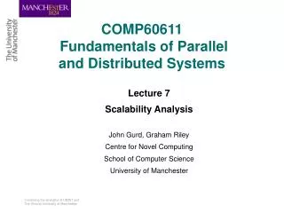
COMP60611Fundamentals of Paralleland Distributed Systems Lecture 4 Introduction to Parallel Algorithms John Gurd, Graham Riley Centre for Novel Computing School of Computer Science University of Manchester

Overview • Generic Properties of Applications • Concrete vs. Abstract Parallelism • Task-Parallelism vs. Data-Parallelism • Two 'Kernel' Algorithms • Elementwise Vector Addition • Vector Sum Reduction • Summary

Generic Properties of Applications • From studies of concurrent systems, we conclude that there are many potential applications, drawn from diverse disciplines and with quite different intrinsic characteristics. • On the other hand, there are some characteristics in common between the applications. For example, scientific simulations often require the use of discrete approximations to continuous domains. • Each application needs an underpinning mathematical model and an algorithmic procedure which 'animates' the model in a fashion suitable for digital computation. • Is it possible to classify the nature of the parallelism that occurs in applications?

Forms of Parallelism • Even from the little we have seen so far, it is obvious that parallelism arises in several different guises. One major distinction lies in the concrete or abstract nature of a specific form of parallelism: • Concrete parallelism occurs wherever its physical characteristics are already fixed (physical nature, time (cost) to invoke, time (cost) to communicate, etc.). This applies mainly at the implementation oriented Levels of Abstraction, primarily at the Computer Level (although one can fix, for example, the run-time system level by choosing a particular process or thread library). • Abstract parallelism occurs wherever there is a logical opportunity for parallel activity, but the physical options have not been fixed. This happens mainly at the application-oriented Levels of Abstraction and at the Program Level before major implementation decisions are made.

Concrete vs. Abstract Parallelism • The concerns surrounding these different kinds of parallelism are clearly distinct: • Abstract parallelism is concerned with finding logical opportunities for parallel activity. The more opportunities that can be found, the greater the prospects for high performance via parallel execution. • Concrete parallelism is concerned with exploiting abstract parallelism in specific implementation circumstances. • In this module we are more interested in the general nature of abstract parallelism (opportunities for concurrency).

Task-Parallelismvs.Data-Parallelism • Perhaps the most practically interesting thing to emerge from our examples so far is the following distinction in styles of parallelism: • Task-parallelism – in which different functions are performed simultaneously, possibly using (part of) the same data; the different functions may take very different times to execute. • Data-parallelism – in which the same function is performed simultaneously, but on different (sets of) data; often, but not always, the function executes in the same time, even though the data values vary. There is further substructure in data-parallelism: experience points to some generic forms which are conveniently introduced using the examples below.

Parallelism • Two very simple examples: • Element-wise vector addition; • Vector sum reduction. • On their own, these are trivial tasks, which we would normally only expect to find embedded as subtasks of some more complex computation. Nevertheless, taken together, they are complex enough to illustrate most of the major issues in parallel computing. They certainly deserve to be treated as a core part of our algorithmic presentation.

Introduction to KernelParallel Algorithms • For each example, we shall investigate: • The work that needs to be done. • The ways in which the necessary work might be done in parallel, ensuring correct results. • Any inherent constraints associated with the resulting parallelism. • How performance might be affected as a result of any choices made. • Remember that we are dealing with abstract parallelism (finding opportunities), so our discussion of concepts such as work and performance will be necessarily vague.

Element-wiseVector Addition • At Algorithm Level, a vector is best thought of as an abstract data type representing a one-dimensional array of elements, all of the same data type. For simplicity, we will use arrays of integer values (this can be generalised with little effort). • The whole vector is normally identified by a user-defined name, while the individual elements of the vector are identified by use of a supplementary integer value, known as the index. The precise semantics of an index value can vary, but a convenient way of viewing it is as an offset, indicating how far away the element is from the first element (or base) of the vector. (In our examples an index of 1 corresponds to the first element.)

Element-wiseVector Addition For our purposes, it is convenient to look at vectors in a diagrammatic form, as follows: vector name A integer elements

Element-wiseVector Addition The task of adding together the elements of two vectors can be drawn as follows: +element-wise -> A and B are input vectors. The result is an output vector.

Element-wiseVector Addition • A simple, sequential algorithm for (element-wise) addition is to form the output vector one element at a time, by running through the elements of the two input vectors, in index order, computing the sum of the pair of input elements at each index point. • The work that has to be done comes in two forms: • Accessing the elements of the vectors (two input vectors and one output vector); and • Computing the sum of each pair of elements. • How might this work be done in parallel? • What range of options are there? • How do these affect performance?

Element-wiseVector Addition • This has been a particularly easy case to study. The work is spread naturally over all the elements of the vectors, each parcel of work is independent of every other parcel of work, and the amount of work in each parcel is the same. • Unfortunately, this kind of parallel work seldom appears on its own, but it is so convenient for parallel systems that it has become known as embarrassingly parallel. Luckily, parallelism in this form frequently does appear as a subtask in algorithms with much more complex structure. • Related examples of this kind of parallel work are scalar multiplication of a vector (or matrix) and general matrix addition (a matrix is a generalisation of the array, used to model phenomena in two or more dimensions).

Vector Sum • Finally, we look at the reduction of a vector into a scalar by summing its elements. For simplicity, we continue to assume integer-valued elements. • The following diagram shows what needs to be done:

Vector Sum • The standard sequential algorithm for this task is to set the output scalar value to zero, and then add the values of the successive elements of the input vector into this 'running total', one-at-a-time. • What scope is there for doing any of this work in parallel? • What range of options are there? • How do these affect performance?

Vector Sum • This example illustrates how parallelism can be found even in tasks whose output is clearly scalar (at least at the level of integers). Because the output is non-parallel, the amount of work that can be done in parallel decreases during the computation. • The standard way of describing this kind of parallel work is divide-and-conquer. In its purest form, this leads to exponentially decreasing parallelism. • Although it is perhaps the most simple of our examples, the presence of a data write conflict leads to the most difficult problems in implementation, as we shall see later.

Algorithmic Core: Summary • Parallel algorithms as-a-whole (i.e. including task-parallelism) boil down to one-or-more of the following three categories: • Complete independence across the data elements (no sharing); embarrassingly parallel. • Shared reads on abstract data elements; implement either by replicating the shared data (then we have independence and it becomes easy!); or by arranging for non-contending memory access (not always easy to achieve). • Shared writes to data elements; in some special cases, we may be able to replicate the shared data (to an extent, but never completely); in the general case, the data must be protected (e.g. using locks) so that access to it is mutually exclusive.

Recap • At Specification Level, a mathematical model of the application is developed; at Algorithm Level, this specification is converted into an appropriate algorithm. Abstract parallelism emerges at both Levels, in both task-parallel and data-parallel forms. • An algorithm is an abstract procedure for solving (an approximation to) the problem at hand; it is based on a discrete data domain that represents (an approximation to) the data domain of the specification. In scientific simulations, where the data domain of the specification is often continuous, it is necessary to develop a 'point-wise' discretisation for the algorithm to work on. Normally, parallelism is then exploited across the elements of the discretised data domain. • The resulting abstract (data-)parallelism appears in three forms: independent, shared reads and shared writes (in increasing order of difficulty to implement).

COMP60611 Fundamentals of Parallel and Distributed Systems