Multiple regression refresher
Multiple regression refresher. Austin Troy NR 245 Based primarily on material accessed from Garson, G. David 2010. Multiple Regression. Statnotes : Topics in Multivariate Analysis. http://faculty.chass.ncsu.edu/garson/PA765/statnote.htm. Purpose.

Multiple regression refresher
E N D
Presentation Transcript
Multiple regression refresher Austin Troy NR 245 Based primarily on material accessed from Garson, G. David 2010. Multiple Regression. Statnotes: Topics in Multivariate Analysis. http://faculty.chass.ncsu.edu/garson/PA765/statnote.htm
Purpose • Y (dependent) as function vector of X’s (independent) • Y=a + b1X1 + b2X2 + ….+bnXn+e • B=0? • Each X adds a dimension • Multiple X’s: effect of Xicontrolling for all other X’s.
Assumptions • Proper specification of the model • Linearity of relationships. Nonlinearity is usually not a problem when the SD of Y is more than SD of residuals. • Normality in error term (not Y) • Same underlying distribution for all variables • Homoscedasticity/Constant variance. Heteroskedacticitymay mean omitted interaction effect. Can use weighted least squares regression or transformation • No outliers. Leverage statistics
Assumptions • Interval, continuous, unbounded data • Non-simultaneity/recursivity: causality one way • Unbounded data • Absence of perfect or high partial multicollinearity • Population error is uncorrelated with each of the independents. "assumption of mean independence”: mean error doesn’t vary with X • Independent observations (absence of autocorrelation) leading to uncorrelated error terms.No spatial/temporal autocorrelation • mean population error=0 • Random sampling
Outputs of regression • Model fit • R2= (1 - (SSE/SST)), where SSE = error sum of squares; SST = total sum of squares • Coefficients table: Intercept, Betas, standard errors, t statistics, p values
Addressing multicollinearity • Intercorrelationof Xs. When excessive, SE of beta coefficients become large, hard to assess relative importance of Xs. • Is a problem when the research purpose includes causal modeling. • Increasing samples size can offset • Options: • Mean center data • Combine variables into a composite variable. • Remove the most intercorrelated variable(s) from analysis. • Use partial least squares, which doesn’t assume no multicollinearity • Ways to check: correlation matrix, Variance inflation Factors. VIF>4 is common rule • VIF from last model diasbp.1 age.1 generaldiet.1 exercise.1 drinker.1 1.136293 1.120658 1.088769 1.101922 1.019268 • However, here is VIF when we regress BMI, age and weight against blood pressure age.1 bmi.1 wt.1 1.13505 3.164127 3.310382
Addressing nonconstantvariance • Bottom graph ideal • Diagnosed with residual plots (or abs resid plot) • Look for funnel shape • Generally suggests the need for: • Generalized linear model • transformation, • weighted least squares or • addition of variables (with which error is correlated) Source: http://www.originlab.com/www/helponline/Origin8/en/regression_and_curve_fitting/graphic_residual_analysis.htm
Considerations: Model specification • U shape or upside down U suggest nonlinear relationship between Xs and Y. • Note: full model residual plots versus partial residual plots • Possible transformations: semi-log, log-log, square root, inverse, power, Box-Cox
Considerations: normality • Normal Quantile plot • Close to normal • Population is skewed to the right (i.e. it has a long right hand tail). • Heavy tailed populations are symmetric, with more members at greater remove from the population mean than in a Normal population with the same standard deviation.


