A Kolmogorov -Smirnov Correlation-Based Filter for Microarray Data
A Kolmogorov -Smirnov Correlation-Based Filter for Microarray Data. Jacek Biesiada Division of Computer Methods, Dep t. of Electrotechnology , The Silesian University of Technology, Katowice, Poland. Włodzisław Duch Dept. of Informatics, Nicola u s Copernicus University, Google: Duch

A Kolmogorov -Smirnov Correlation-Based Filter for Microarray Data
E N D
Presentation Transcript
A Kolmogorov-Smirnov Correlation-Based Filterfor Microarray Data Jacek Biesiada Division of Computer Methods, Dept. ofElectrotechnology, The Silesian University of Technology, Katowice, Poland. Włodzisław Duch Dept. of Informatics, Nicolaus Copernicus University, Google: Duch ICONIP 2007
Motivation • Attention: is a basic cognitive skill, without focus on relevant information cognition would not be possible. • In natural perception (vision, auditory scenes, tactile signals) large number of features may be dynamically selected depending on the task. • Large feature spaces: (genes, proteins, chemistry, etc): different features are relevant. • Filters will leave large number of potentially relevant features. • Redundancy should be removed! • Fast filters with removal of redundancy are needed! • Microarrays: popular testing ground, although not reliable due to small number of samples. • Goal: fast filter + redundancy removal + tests on microarray data to identify problems.
Microarray matrices Genes in rows, samples in columns, DNA/RNA type
Selection of information • Find relevant information: • discard attributes that do not contain information. • use weights to express the relative importance. • create new, more informative attributes. • reduce dimensionality aggregating information. • Ranking: treat each feature as independent. • Selection: search for subsets, remove redundant. • Filters: universal criteria, model-independent. • Wrappers: criteria specific for data models are used. • Frapper: filter + wrapper in the final stage. • Redfilapper: redundancy removal + filter + wrapper. • Create fast redfilapper.
Filters & Wrappers Filter approach for data D: • define your problem C, for example assignment of class labels; • define an index of relevance for each feature Ji=J(Xi)=J(Xi|D,C) • calculate relevance indices for all features and order Ji1 Ji2 .. Jid • remove all features with relevance below threshold J(Xi) < tR • Wrapper approach: • select predictor Pand performance measure J(D|X)=P(Data|X). • define search scheme: forward, backward or mixed selection. • evaluate starting subset of features Xs, ex. single best or all features • add/remove feature Xi, accept new set Xs{Xs+Xi} if P(Data|Xs+Xi)>P(Data|Xs)
Information gain Information gained by considering the joint probability distribution p(C, f) is a difference between: • A feature is more important if its information gain is larger. • Modifications of the information gain, used as criteria in some decision trees, include:IGR(C,Xj) = IG(C,Xj)/I(Xj)the gain ratio IGn(C,Xj) = IG(C,Xj)/I(C)an asymmetric dependency coefficient DM(C,Xj) = 1-IG(C,Xj)/I(C,Xj)normalized Mantaras distance
Information indices Information gained considering attribute Xj and classes C together is also known as ‘mutual information’, equal to the Kullback-Leibler divergence between joint and product probability distributions: Entropy distance measure is a sum of conditional information: Symmetrical uncertainty coefficient is obtained from entropy distance:
Purity indices Many information-based quantities may be used to evaluate attributes.Consistency or purity-based indices are one alternative. For selection of subset of attributes F={Xi} the sum runs over all Cartesian products, or multidimensional partitions rk(F). Advantages: simplest approach both ranking and selection Hashing techniques are used to calculate p(rk(F))probabilities.
Correlation coefficient Perhaps the simplest index is based on the Pearson’s correlation coefficient (CC) that calculates expectation values for product of feature values and class values: For feature values that are linearly dependent correlation coefficient is +1or -1; for complete independence of class and Xj distribution CC= 0. How significant are small correlations? It depends on the number of samples n. The answer (see Numerical Recipes www.nr.com) is given by: For n=1000 even small CC=0.02 gives P ~ 0.5, but for n=10 such CC gives only P ~0.05.
F-score Mutual information is based on Kullback-Leibler distance, any distance measure between distributions may also be used, ex. Jeffreys-Matusita with pooled variance calculated from For two classes F = t2 or t-score. Many other such (dis)similarity measures exist. Which is the best? In practice they all are similar, although accuracy of calculation of indices is important; relevance indices should be insensitive to noise and unbiased in their treatment of features with many values.
State-of-the-art methods 1. FCBF, Fast Correlation-Based Filter (Yu & Liu 2003). • Compare feature-class Ji=SU(Xi,C) and feature-feature SU(Xi,Xj); • rank features Ji1 ≥ Ji2≥ Ji3... ≥ Jim ≥ min threshold. • Compare feature Xito all Xjlower in ranking, • if SU(Xi, Xj) ≥ SU(C,Xi) then Xi is redundant and is removed. • ConnSF, Consistency features selection (Dash, Liu, Motoda 2000). • Inconsistency JI(S) for discrete valued feature S isJI(S) = n − n(C). where a subset of features S with values VS appears n times in the data, most often n(C) times with the label of class C. • Total inconsistency count = sum of all the inconsistency counts for all distinct patterns of a feature subsets S. • Consistency = the least inconsistency count. • 3. CorrSF (Hall 1999), based on correlation coefficient with 5 step backtracking.
Kolmogorov-Smirnov test Are distributions of values of two different features roughly equal? If yes, one is redundant. • Discretization process creates k clusters (vectors from roughly the same class), each typically covering similar range of values. • A much larger number of independent observation n1, n2> 40 are taken from the two distributions, measuring frequencies of different classes. • Based on the frequency table the empirical cumulative distribution functions F1iand F2iare constructed. • λ(K-S statistics) is proportional to the largest absolute difference of |F1i − F2i|, and if λ < λα distributions are equal:
KS-CBS • Kolmogorov-Smirnov Correlation-Based Selection algorithm. Relevance analysis Order features according to the decreasing values of relevance indices creating S list. Redundancy analysis Initialize Fi to the first feature in the S list. Use K-S test to find and remove from S all features for which Fi forms an approximate redundant cover C(Fi). Move Fi to the set of selected features, take as Fi the next remaining feature in the list. Repeat step 3 and 4 until the end of the S list.
3 Datasets • Leukemia: training 38 bone marrow samples (27 of the ALL and 11 of the AML type), using 7129 probes from 6817 human genes; 34 test samples are provided, with 20 ALL and 14 AML cases. Too small for such split, • Colon Tumor: 62 samples collected from colon cancer patients, with 40 biopsies from tumor areas (labelled as “negative") and 22 from healthy parts of the colons of the same patients. 2000 out of around 6500 genes were pre-selected, based on the confidence in the measured expression levels. • Diffuse Large B-cell Lymphoma [DLBCL]: two distinct types of diffuse large lymphoma B-cells (most common subtype of non-Hodgkin’s lymphoma); 47 samples, 24 from “germinal centre B-like" group, 23 are from “activated B-like" group, 4026 genes.
Discretization & classifiers For comparison of information selection techniques simple discretization of gene expression levels into 3 intervals is used. Variance σ, mean μ, discrete values -1, 0, +1 for (-,μ − σ/2), [μ − σ/2 , μ + σ/2 ], (μ+ σ/2, +) Represents under-expression, baseline and over-expression of genes. Results after such discretization are in some cases significantly improved and are given in parenthesis in the tables below. Classifiers used: • C4.5 decision tree (Weka), • Naive Bayes with single Gaussian kernel, or discretized prob., • k-NN, or 1 nearest neighbor algorithm (Ghostminer implementation) • Linear SVM with C = 1 (also GM)
No. of features selected • For standard a=0.05 confidence level for redundancy rejection relatively large number of features is left for Leukemia. • Even for a=0.001 confidence level 47 features are left; best to optimize it by wrapper. • A larger number of feature may lead to more reliable “profile” (ex. by chance one gene in Leukemia gets 100% on training). • Large improvements up to 30% in accuracy, with small number of samples statistical significance is ~5%. • Discretization improves results in most cases.
Leukemia: Bayes rules Top: test, bottom: train; green = p(C|X) for Gaussian-smoothed density with s=0.01, 0.02, 0.05, 0.20 (Zyxin).
Leukemia SVM LVO Problems with stability
Leukemia boosting 3 best genes, evaluation using bootstrap.
Conclusions • K-S CBS algorithm combines relevance indices (F-measure, SUC or other index) to rank and reduce the number of features, and uses Kolmogorov-Smirnov test to reduce the number of features further. • It is computationally efficient and gives quite good results. • Variants of this algorithm may identify approximate redundant covers for consecutive features Xi and leave in the S set only the one that gives best results. • Problems with stability of solutions for small and large data! no significant difference between many feature selection methods. • Frapper selects on training those that are helpful in O(m) steps, stabilizes LOO results a bit, but it is not a complete solution. • Will anything work reliably for microarray feature selection? Are results published so far worth anything?