Download

1 / 36
360 likes | 585 Vues
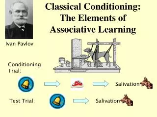
Classical Conditioning (also Pavlovian / Respondent Conditioning). Basic principles of classical conditioning. A tribute to Ivan Pavlov 1849 - 1936. The experiment. Before An unconditional stimulus (US) elicits an unconditional response (UR). Dry food in the dog's mouth elicits salivation

E N D
Classical Conditioning(also Pavlovian / Respondent Conditioning)
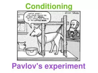
Basic principles of classical conditioning A tribute to Ivan Pavlov 1849 - 1936
The experiment • Before • An unconditional stimulus (US) elicits an unconditional response (UR). Dry food in the dog's mouth elicits salivation • A conditional stimulus (CS) initially elicits an orienting response different from the UR. • During • The CS is paired with the US. • A short CS--US time interval • A relatively long US--US interval • After • The CS elicits a Conditional Response (CR). • The orienting response to the CS has habituated
PAVLOVIAN PARADIGM unconditional stimulus unconditional response elicits UCR UCS elicits CR CS conditional stimulus conditional response But what does mean?
CS CS CS CS US US US US Temporal Relations and Conditioning Delay Conditioning Trace Conditioning Simultaneous Conditioning Backward Conditioning
BASIC PHENOMENA • ACQUISITION • EXTINCTION • STIMULUS CONTROL
Pavlov’s Law of Strength • Number of trials rule: The greater the number of CS-US pairings, the stronger the CR. • CS intensity rule: More intense CS's increase the rate of growth of the CR but do not seem to affect its asymptote. • US Intensity rule: More intense US's affect both the rate of growth and the asymptote of the CR. • CS-US interval rule: Longer CS-US intervals yield lower asymptotes of the CR. This rule highlights the importance of contiguity in classical conditioning. • CS-US contingency rule: The asymptote of the CR increases with the correlation between the CS and the US. This rule highlights the importance of contingency in classical conditioning.
Is key element S-S (CS – UCS) or S-R (CS – UCR) relationship? • Sensory preconditioning • Idea of stimulus substitution
What are the necessary and sufficient conditions for Pavlovian conditioning to occur? • Response Class • Temporal Relations • Contingency
[SOME] CHALLENGES TO CONTIGUITY • 1. OVERSHADOWING • 2. BLOCKING • 3. SERIAL STIMULUS SELECTION • 4. CONDITIONAL INHIBITION • 5. CS PRE-EXPOSURE EFFECT (latent inhibition) • 6 UCS PRE-EXPOSURE EFFECT • 7. CONTIGUITY versus CORRELATION
Respondent Contingencies • Standard Procedure • P(UCS|CS) = 1 ; P(UCS|~CS) = 0 • Partial Reinforcement • 0 < P(UCS|CS) < 1 ; P(UCS|~CS) = 0 • Random Control • 0 < P(UCS|CS) = P(UCS|~CS) • Inhibitory CS • 0 < P(UCS|CS) < P(UCS|~CS) Pavlovian Conditioning
Contingency Table UCS ~UCS #UCSCS = A # CS = A + B P(UCS|CS) = A / (A+B) CS B A+B A ~CS D C+D C A+C B+D N |AD - BC| (A+B)(C+D)(A+C)(B+D) = Pavlovian Conditioning
Staddon’s Data Pavlovian Conditioning
Contingencies and Staddon’s Data SH ~SH = 20/30 = 2/3 = 10/30 = 1/3 = 10/30 = 1/3 = 20/30 = 2/3 P(S) P(~S) P(SH) P(~SH) 10 20 S 10 012 011 10 ~S 10 0 022 021 30 10 20 Pavlovian Conditioning
Contingencies and Staddon’s Data If S and SH were independent (“random control”): P (SH|S) = P (SH) or P (SH S) = P (SH) P(S) By definition: P (SH|S) = P (SH S) = #(SH and S) P(S) #S = 10/20 = 1/2 But: P (SH) = 10/30 = 1/3 So: P (SH|S) ≠ P (SH). Also, P (SH S) ≠ P (SH) P(S) 10/30 = 1/3 ≠ (1/3)(2/3) = 2/9 Pavlovian Conditioning
= X²1df= │011022 – 012021│ • N (011 + 012)(021 + 022)(011 + 021)(012 +022) Recall X² test for independence in contingency table with observed frequencies 0ij rc i=1 j=1 Where the Eij’s are the Expected Frequencies X²1df = (0ij – Eij) ² Eij For a 2 x 2 Table X²1df = N │011022 – 012021│² (011 + 012)(021 + 022)(011 + 021)(012 +022) Pavlovian Conditioning
For a 2 x 2 Table Χ²1df = N │011022 – 012021│² (011 + 012)(021 + 022)(011 + 021)(012 +022) SH ~SH E11 = (011 + 012)(011 + 021) N E12 = (011 + 012)(012 + 022) N E21 = (021 + 022)(011 + 021) N E22 = (021 + 022)(012 + 022) N S 011 + 012 012 011 021 022 021 + 022 ~S N 012 + 022 011 + 021 Pavlovian Conditioning
X1² = (13.33 – 10)² + (10 - 6.67)² 13.33 6.67 + (10 – 6.67)² + (3.33 -0)² 6.67 3.33 = 7.486 ≈ 7.5 X².95 = 3.84 1df = │(10(0) – (10)(10) │= 100 = 0.5 (20)(10)(20)(10) (20)(10) ² = 0.25 = X1² / 30, so X1² = 7.5 as above. S and Shock are not independent • For Staddon’s Data, the table is: 011 = 10 E11 = 13.33 012 = 10 E12 = 6.67 20 022 = 0 E22 = 3.33 021 = 10 E21 = 6.67 10 30 10 20 Pavlovian Conditioning
cs S = Rcs Rcs+ Rcs cs cs S = 0.0 S = 0.5 Pavlovian Conditioning
P(UCS|CS) = P(UCS|~CS) = P(UCS~CS) = # (UCS~CS) P(~CS) # ~CS [P(CS) > 0] ~CS E UCSCS UCS~CS ~CS = E – CS = Context P(UCS|CS) = 1- P(~UCS|CS) P(UCS|~CS) = 1- P(~UCS|~CS) ~UCS Pavlovian Conditioning
What are some characteristics of a good model? Variables well-described and manipulatable. Accounts for known results and able to predict non-trivial results of new experiments. Dependent variable(s) predicted in at least relative magnitude and direction. Parsimonious (i.e., minimum assumptions for maximum effectiveness).
STEPS IN MODEL BUILDING • IDENTIFICATION: WHAT’S THE QUESTION? • ASSUMPTIONS: WHAT’S IMPORTANT; WHAT’S NOT? • CONSTRUCTION: MATHEMATICAL FORMULATION • ANALYSIS: SOLUTIONS • INTERPRETATION: WHAT DOES IT MEAN? • VALIDATION: DOES IT ACCORD WITH KNOWN DATA? • IMPLEMENTATION: CAN IT PREDICT NEW DATA?
PRINCIPAL THEORETICAL VARIABLE: ASSOCIATIVE STRENGTH, V
ASSUMPTIONS 1. When a CS is presented its associative strength, Vcs, may increase (CS+), decrease (CS-), or remain unchanged. 2. The asymptotic strength () of association depends on the magnitude (I) of the UCS: = f (UCSI). 3. A given UCS can support only a certain level of associative strength, . 4. In a stimulus compound, the total associative strength is the algebraic sum of the associative strength of the components. [ex. T: tone, L: light. VT+L =VT + VL] 5. The change in associative strength, V, on any trial is proportional to the difference between the present associative strength, Vcs, and the asymptotic associative strength, .
R-W APPLIED TO VARIOUS EFFECTS ACQUISITION 2. EXTINCTION 3. OVERSHADOWING 4. BLOCKING 5. CONDITIONAL INHIBITION
Contiguity in R-W Model If P(UCS|CS) = P(UCS|~CS), we really have CS = CS + CTX and ~CS = CTX. Then: P(UCS|CS + CTX) = P(UCS|CTX) V (CS + CTX) = VCS + VCTX (R-W axiom) V CS = V (CS +CTX) = VCS + VCTX but: V CTX = V ~CS so: V (CS + CTX) = V CS + V~CS = 0 No significant conditioning occurs to the CS Pavlovian Conditioning