Gradient Analysis Approach to Ordination
Gradient Analysis Approach to Ordination. Models of Species Response to Gradients. Models of Species Response. There are (at least) two models:- Linear - species increase or decrease along the environmental gradient


Gradient Analysis Approach to Ordination
E N D
Presentation Transcript
Models of Species Response There are (at least) two models:- • Linear - species increase or decrease along the environmental gradient • Unimodal - species rise to a peak somewhere along the environmental gradient and then fall again
Alpha and Beta Diversity • alpha diversity is the diversity of a community (either measured in terms of a diversity index or species richness) • beta diversity (also known as ‘species turnover’ or ‘differentiation diversity’) is the rate of change in species composition from one community to another along gradients; gamma diversity is the diversity of a region or a landscape.
Indirect Gradient Analysis • Environmental gradients are inferred from species data alone • Three methods: • Principal Component Analysis - linear model • Correspondence Analysis - unimodal model • Detrended CA - modified unimodal model
Site A B C D E F SpeciesPrunus serotina 6 3 4 6 5 1Tilia americana2 0 7 0 6 6Acer saccharum0 0 8 0 4 9Quercus velutina0 8 0 8 0 0Juglans nigra3 2 3 0 6 0 Reciprocal Averaging
Site A B C D E F Species ScoreSpecies Iteration 1Prunus serotina 6 3 4 6 5 11.00Tilia americana2 0 7 0 6 60.63Acer saccharum0 0 8 0 4 90.63Quercus velutina0 8 0 8 0 00.18Juglans nigra3 2 3 0 6 00.00 Iteration11.00 0.00 0.86 0.60 0.62 0.99SiteScore Reciprocal Averaging
Site A B C D E F Species ScoreSpecies Iteration 12Prunus serotina 6 3 4 6 5 1 1.00 0.68Tilia americana2 0 7 0 6 6 0.63 0.84Acer saccharum0 0 8 0 4 9 0.63 0.87Quercus velutina0 8 0 8 0 0 0.18 0.30Juglans nigra3 2 3 0 6 0 0.00 0.67 Iteration 1 1.00 0.00 0.86 0.60 0.62 0.99Site20.65 0.00 0.88 0.05 0.78 1.00Score Reciprocal Averaging
Site A B C D E F Species ScoreSpecies Iteration 1 23Prunus serotina 6 3 4 6 5 1 1.00 0.68 0.50Tilia americana2 0 7 0 6 6 0.63 0.84 0.86Acer saccharum0 0 8 0 4 9 0.63 0.87 0.91Quercus velutina0 8 0 8 0 0 0.18 0.30 0.02Juglans nigra3 2 3 0 6 0 0.00 0.67 0.66 Iteration 1 1.00 0.00 0.86 0.60 0.62 0.99Site 2 0.65 0.00 0.88 0.05 0.78 1.00Score30.60 0.01 0.87 0.00 0.78 1.00 Reciprocal Averaging
Site A B C D E F Species ScoreSpecies Iteration 1 2 3 9Prunus serotina 6 3 4 6 5 1 1.00 0.68 0.50 0.48Tilia americana2 0 7 0 6 6 0.63 0.84 0.86 0.85Acer saccharum0 0 8 0 4 9 0.63 0.87 0.91 0.91Quercus velutina0 8 0 8 0 0 0.18 0.30 0.02 0.00Juglans nigra3 2 3 0 6 0 0.00 0.67 0.66 0.65 Iteration 1 1.00 0.00 0.86 0.60 0.62 0.99Site 2 0.65 0.00 0.88 0.05 0.78 1.00Score 3 0.60 0.01 0.87 0.00 0.78 1.0090.59 0.01 0.87 0.00 0.78 1.00 Reciprocal Averaging
Site A C E B D F Species SpeciesScoreQuercus velutina8 8 0 0 0 0 0.004Prunus serotina6 3 6 5 4 10.477Juglans nigra0 2 3 6 3 0 0.647Tilia americana0 0 2 6 7 6 0.845Acer saccharum0 0 0 4 8 9 0.909Site Score0.000 0.008 0.589 0.778 0.872 1.000 Reordered Sites and Species
3 2 1 0 CA2 -1 -2 -3 -4 -2 0 2 4 CA1 CA - unimodal model Tardigrada + Rotifera + Nematoda + Annelida + + + Insecta Protozoa + + + Cladocera Turbellaria + Copepoda
The Arch Effect • What is it? • Why does it happen? • What should we do about it?
Long Gradients A B C D
Direct Gradient Analysis • Environmental gradients are constructed from the relationship between species environmental variables • Three methods: • Redundancy Analysis - linear model • Canonical (or Constrained) Correspondence Analysis - unimodal model • Detrended CCA - modified unimodal model
Partial Analyses • Remove the effect of covariates • variables that we can measure but which are of no interest • e.g. block effects, start values, etc. • Carry out the gradient analysis on what is left of the variation after removing the effect of the covariates.
Randomisation Example Model: cca(formula = dune ~ Moisture + A1 + Management, data = dune.env) Df Chisq F N.Perm Pr(>F) Model 7 1.1392 2.0007 200 < 0.005 *** Residual 12 0.9761 Signif. codes: 0 *** 0.001 ** 0.01 * 0.05