Download
1 / 45
470 likes | 748 Vues
Ion Heating in the Solar Corona. Steven R. Cranmer Harvard-Smithsonian Center for Astrophysics. Ion Heating in the Solar Corona. Outline: 1. Remote-sensing (UV coronagraph spectroscopy) 2. Follow the ion cyclotron trail to. . . 3. Anisotropic MHD turbulence, and . . .

E N D
Ion Heating in the Solar Corona Steven R. CranmerHarvard-Smithsonian Center for Astrophysics
Ion Heating in the Solar Corona Outline: 1. Remote-sensing (UV coronagraph spectroscopy) 2. Follow the ion cyclotron trail to. . . 3. Anisotropic MHD turbulence, and . . . 4. The macroscopic coronal heating problem Steven R. CranmerHarvard-Smithsonian Center for Astrophysics
On-disk vs. off-limb observations • On-disk measurements help reveal basal coronal heating & lower boundary conditions for solar wind. • Off-limb measurements (in the solar wind “acceleration region” ) allow dynamic non-equilibrium plasma states to be followed as the asymptotic conditions at 1 AU are gradually established. Occultation is required because extended corona is 5 to 10 orders of magnitude less bright than the disk! Spectroscopy provides detailed plasma diagnostics that imaging alone cannot.
Mirror motions select height • UVCS “rolls” independently of spacecraft • 2 UV channels: • 1 white-light polarimetry channel LYA (120–135 nm) OVI (95–120 nm + 2nd ord.) The UVCS instrument on SOHO • SOHO (the Solar and Heliospheric Observatory) was launched in Dec. 1995 with 12 instruments probing solar interior to outer heliosphere. • The Ultraviolet Coronagraph Spectrometer (UVCS) measures plasma properties of coronal protons, ions, and electrons between 1.5 and 10 solar radii. • Combines occultation with spectroscopy to reveal the solar wind’s acceleration region. slit field of view:
Emission line diagnostics • Off-limb photons formed by both collisional excitation/de-excitation and resonant scattering of solar-disk photons. • Net Doppler shifts (from the known “rest wavelength”) indicate the bulk flow speed alongthe line-of-sight. • The widths of profiles tell us about random motions along the line-of-sight (i.e., temperature) • The total intensity (i.e., number of photons) tells us mainly about the density of atoms, but for resonant scattering there’s also another “hidden” Doppler effect that tells us about motions perpendicular to the line-of-sight.
UVCS results: solar minimum (1996-1997) • UVCS led to new views of the collisionless nature of solar wind acceleration. • In coronal holes, heavy ions (e.g., O+5) both flow faster and are heated hundreds of times more strongly than protons and electrons, and have anisotropic velocity distributions. Kohl et al. (1995, 1997, 1998, 1999, 2006); Cranmer et al. (1999); Cranmer (2000, 2001, 2002)
Alfven wave’s oscillating E and B fields ion’s Larmor motion around radial B-field Ion cyclotron waves in the corona • UVCS observations have rekindled theoretical efforts to understand heating and acceleration of the plasma in the (collisionless!) acceleration region of the wind. • Ion cyclotron waves (10 to 10,000 Hz) suggested as a natural energy source that can be tapped to preferentially heat & accelerate heavy ions. • Dissipation of these waves produces diffusion in velocity space along contours of ~constant energy in the frame moving with wave phase speed: lower Z/A faster diffusion
Where do cyclotron waves come from? (1) Base generation by, e.g., “microflare” reconnection in the lanes that border convection cells (e.g., Axford & McKenzie 1997). (2) Secondary generation: low-frequency Alfven waves may be converted into cyclotron waves gradually in the corona. Both scenarios have problems . . .
“Opaque” cyclotron damping (1) • If high-frequency waves originate only at the base of the corona, extended heating must “sweep” across the frequency spectrum. • For proton cyclotron resonance only (Tu & Marsch 1997):
“Opaque” cyclotron damping (2) • However, minor ions can damp the waves as well: • Something very similar happens to resonance-line photons in winds of super-luminous massive stars! • Cranmer (2000, 2001) computed “tau” for >2500 ion species. • If cyclotron resonance is indeed the process that energizes high-Z/A ions, the wave power must be replenished continually throughout the extended corona.
Charge/mass dependence • Assuming enough “replenishment” (via, e.g., turbulent cascade?) to counteract local damping, the degree of preferential ion heating depends on the assumed distribution of wave power vs. frequency (or parallel wavenumber): O VI (O+5) measurement used to normalize heating rate. Mg X (Mg+9) showed a much narrower line profile (despite being so close to O+5 in its charge-to-mass ratio)!
Future diagnostics: additional ions? • For one specific choice of the power-law index, we can also include either: enough “local” damping (depending on “tau”) or enough Coulomb collisions to produce the narrower Mg+9 profile widths . . . (Cranmer 2002, astro-ph/0209301)
Aside: two other (non-cyclotron) ideas . . . • If the corona is filled with “thin” MHD shocks, an ion’s upstream v becomes oblique to the downstream field. Some gyro-motion arises before the ion “knows” it! (Lee & Wu 2000). • Kinetic Alfven waves with nonlinear amplitudes generate E fields that can scatter ions non-adiabatically and heat them perpendicularly (Voitenko & Goossens 2004).
Where to go from here? • The “free parameters” in all of the above ideas depend on the macroscopic properties of the motions (waves? shocks? turbulent eddies?) that feed the microscopic kinetic scales. • Can a turbulent cascade create ion cyclotron waves?
MHD turbulence • It is highly likely that somewhere in the outer solar atmosphere the fluctuations become turbulent and cascade from large to small scales:
MHD turbulence • It is highly likely that somewhere in the outer solar atmosphere the fluctuations become turbulent and cascade from large to small scales: • With a strong background field, it is easier to mix field lines (perp. to B) than it is to bend them (parallel to B). • Also, the energy transport along the field is far from isotropic: Z– Z+ Z– (e.g., Matthaeus et al. 1999; Dmitruk et al. 2002)
freq. horiz. wavenumber horiz. wavenumber Does this create ion cyclotron waves? • Preliminary models say “probably NO” in the extended corona. (At least not in a straightforward way!) • In the corona, RMHD cascade creates “kinetic Alfven waves” with high k that heat electrons (T >> T ) when they damp linearly.
freq. horiz. wavenumber horiz. wavenumber something else? Does this create ion cyclotron waves? • Preliminary models say “probably NO” in the extended corona. (At least not in a straightforward way!) • In the corona, RMHD cascade creates “kinetic Alfven waves” with high k that heat electrons (T >> T ) when they damp linearly. How then are the ions heated & accelerated? • Nonlinear instabilities that locally generate high-freq. waves (Markovskii 2004)? • Coupling with fast-mode waves that can cascade to high-freq. (Chandran 2006)? • KAW damping leads to electron beams, further (Langmuir) turbulence, and Debye-scale electron phase space holes, which heat ions perpendicularly via “collisions” (Ergun et al. 1999; Cranmer & van Ballegooijen 2003)? cyclotron resonance-like phenomena MHD turbulence
Where to go from there? • We can compute a net heating rate from the cascade, even if we don’t know how the energy gets “partitioned” to the different particle species.
Start with the “lower boundary” • Photosphere displays convective motion on a broad range of time/space scales: β << 1 β ~ 1 β > 1
Open flux tubes: global model • Photospheric flux tubes are shaken by an observed spectrum of horizontal motions. • Alfvén waves propagate along the field, and partly reflect back down (non-WKB). • Nonlinear couplings allow a (mainly perpendicular) cascade, terminated by damping. (Heinemann & Olbert 1980; Hollweg 1981, 1986; Velli 1993; Matthaeus et al. 1999; Dmitruk et al. 2001, 2002; Cranmer & van Ballegooijen 2003, 2005; Verdini et al. 2005; Oughton et al. 2006; many others!)
“The kitchen sink” • Cranmer, van Ballegooijen, & Edgar (2007) computed self-consistent solutions of waves & background one-fluid plasma state along various flux tubes... going from the photosphere to the heliosphere. (astro-ph/0703333) • Ingredients: • Alfvén waves: non-WKB reflection with full spectrum, turbulent damping, wave-pressure acceleration • Acoustic waves: shock steepening, TdS & conductive damping, full spectrum, wave-pressure acceleration • Radiative losses: transition from optically thick (LTE) to optically thin (CHIANTI + PANDORA) • Heat conduction: transition from collisional (electron & neutral H) to collisionless “streaming”
Coronal heating emerges naturally . . . Ulysses SWOOPS T (K) Goldstein et al. (1996) reflection coefficient
More plasma diagnostics Better understanding Conclusions • UV coronagraph spectroscopy has led to fundamentally new views of the collisionless acceleration regions of the solar wind. • Theoretical advances in MHD turbulence continue to “feed back” into global models of the solar wind. • The extreme plasma conditions in coronal holes (T ion>> Tp > Te ) have guided us to discard some candidate processes, further investigate others, and have cross-fertilized other areas of plasma physics & astrophysics. • Next-generation observational programs are needed for conclusive “constraints.” For more information: http://www.cfa.harvard.edu/~scranmer/
Alfvén wave reflection • At photosphere: empirically-determined frequency spectrum of incompressible transverse motions (from statistics of tracking inter-granular bright points) • At all larger heights: self-consistent distribution of outward (z–) and inward (z+) Alfvenic wave power, determined by linear non-WKB transport equation: refl. coeff = |z+|2/|z–|2 TR
SUPERSONIC coronal heating: subsonic region is unaffected. Energy flux has nowhere else to go: M same, u vs. SUBSONIC coronal heating: “puffs up” scale height, draws more particles into wind: M u Why is the fast/slow wind fast/slow? • Several ideas exist; one powerful one relates flux tube expansion to wind speed (Wang & Sheeley 1990). Physically, the geometry determines location of Parker critical point, which determines how the “available” heating affects the plasma: Banaszkiewicz et al. (1998)
Magnetic flux tubes • Vary the magnetic field, but keep lower-boundary parameters fixed. “active region” fields
Fast/slow wind diagnostics • The wind speed & density at 1 AU behave mainly as observed. Cascade efficiency: n=1 n=2 Ulysses SWOOPS Goldstein et al. (1996)
Fast/slow wind diagnostics • To compare modeled wave amplitudes with in-situ fluctuations, knowledge about the spectrum is needed . . . • “e+”: (in km2 s–2 Hz–1 ) defined as the Z– energy density at 0.4 AU, between 10–4 and 2 x 10⁻⁴ Hz, using measured spectra to compute fraction in this band. Helios (0.3–0.5 AU) Tu et al. (1992) Cranmer et al. (2007)
Fast/slow wind diagnostics • Frozen-in charge states • FIP effect (using Laming’s 2004 theory) Ulysses SWICS Cranmer et al. (2007)
Progress towards a robust “recipe” Not too bad, but . . . • Because of the need to determine non-WKB (nonlocal!) reflection coefficients, it may not be easy to insert into global/3D MHD models. • Doesn’t specify proton vs. electron heating (they conduct differently!) • Does turbulence generate enough ion-cyclotron waves to heat the minor ions? • Are there additional (non-photospheric) sources of waves / turbulence / heating for open-field regions? (e.g., flux cancellation events) (B. Welsch et al. 2004)
“Anisotropic” cascade • Traditional (RMHD-like) nonlinear terms have a cascade energy flux that gives phenomenologically simple heating: • We use a generalization based on unequal wave fluxes along the field . . . Z– Z+ • n = 1: usual “golden rule;” we also tried n=2. Z– (e.g., Pouquet et al. 1976; Dobrowolny et al. 1980; Zhou & Matthaeus 1990; Hossain et al. 1995; Dmitruk et al. 2002)
Coronal holes: over the solar cycle • Even though large coronal holes have similar outflow speeds at 1 AU (>600 km/s), their acceleration (in O+5) in the corona is different! (Miralles et al. 2001) Solar minimum: Solar maximum:
Doppler dimming & pumping • After H I Lyman alpha, the O VI 1032, 1037 doublet are the next brightest lines in the extended corona. • The isolated 1032 line Doppler dims like Lyman alpha. • The 1037 line is “Doppler pumped” by neighboring C II line photons when O5+ outflow speed passes 175 and 370 km/s. • The ratio R of 1032 to 1037 intensity depends on both the bulk outflow speed (of O5+ ions) and their parallel temperature. . . • The line widths constrain perpendicular temperature to be > 100 million K. • R < 1 implies anisotropy!
Thin tubes merge into supergranular funnels Peter (2001) Tu et al. (2005)
Resulting wave amplitude (with damping) • Transport equations solved for 300 “monochromatic” periods (3 sec to 3 days), then renormalized using photospheric power spectrum. • One free parameter: base “jump amplitude” (0 to 5 km/s allowed; 3 km/s is best)
Turbulent heating rate • Solid curve: predicted Qheat for a polar coronal hole. • Dashed RGB regions: empirical estimates of heating rate of primary plasma (models tuned to match conditions at 1 AU). • What is really needed are direct measurements of the plasma (atoms, ions, electrons) in the acceleration region of the solar wind!
Streamers: open and/or closed? Wang et al. (2000) • High-speed wind: strong connections to the largest coronal holes hole/streamer boundary (streamer “edge”) streamer plasma sheet (“cusp/stalk”) small coronal holes active regions (some with streamer cusps) • Low-speed wind: still no agreement on the full range of coronal sources:
The Need for Better Observations • Even though UVCS/SOHO has made significant advances, • We still do not understand the physical processes that heat and accelerate the entire plasma (protons, electrons, heavy ions), • There is still controversy about whether the fast solar wind occurs primarily in dense polar plumes or in low-density inter-plume plasma, • We still do not know how and where the various components of the variable slow solar wind are produced (e.g., “blobs”). (Our understanding of ion cyclotron resonance is based essentially on just one ion!) UVCS has shown that answering these questions is possible, but cannot make the required observations.
Coronal heating mechanisms • So many ideas, taxonomy is needed! (Mandrini et al. 2000; Aschwanden et al. 2001) • Where does the mechanical energy come from? • How rapidly is this energy coupled to the coronal plasma? • How is the energy dissipated and converted to heat? vs. waves shocks eddies (“AC”) twisting braiding shear (“DC”) vs. interact with inhomog./nonlin. turbulence reconnection collisions (visc, cond, resist, friction) or collisionless
AC versus DC heating? • Waves cascade into MHD turbulence (eddies), which tends to: • break up into thin reconnecting sheets on its smallest scales. • accelerate electrons along the field and generate currents. • Coronal current sheets are unstable in a variety of ways to growth of turbulent motions which may dominate the energy loss & particle acceleration. e.g., Dmitruk et al. (2004) • Turbulence may drive “fast” reconnection rates (Lazarian & Vishniac 1999), too. Onofri et al. (2006)
The solar atmosphere Heating is everywhere . . . . . . and everything is in motion
“New stars” 1572: Tycho’s supernova 1600: P Cygni outburst (“Revenante of the Swan”) 1604: Kepler’s supernova in “Serepentarius” First observations of stellar outflows ? • Coronae & Aurorae seen since antiquity . . .
One-page stellar wind physics • Momentum conservation: To sustain a wind, /t = 0 , and RHS must be “tuned:” • Energy conservation: • Extended corona & cool-star wind • Transition region & low corona • Chromosphere: heating rad. losses • Photosphere (& most of hot-star wind)