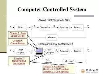
Computer Controlled System
Computer Controlled System. Chapter 7 State Space Design. Chapter 6 Classic Design. Chapter 2 Sampling and construction. Chapter 3 Z transform Chapter 4 CCS Modelling Chapter 5 CCS Analyzing. Chapter 2 Sampling and Construction. 1. The steps of the processes of A/D and D/A

Computer Controlled System
E N D
Presentation Transcript
Computer Controlled System Chapter 7 State Space Design Chapter 6 Classic Design Chapter 2 Sampling and construction Chapter 3 Z transform Chapter 4 CCS Modelling Chapter 5 CCS Analyzing
Chapter 2 Sampling and Construction 1. The steps of the processes of A/D and D/A 2. Types of Signals in CCS • Analog signal/ digital signal/ sampled signal 3. Mathematical description of sampling signal • Time domain / frequency domain 4. Sampling theorem (s 2max, N= s /2) 5. Reconstruction • Ideal reconstruction/non-ideal reconstruction/ZOH
Chapter 2 Sampling and Construction • Sample-and-hold circuit • A-D converter Quantization • Coding 1. The steps of the processes of A/D and D/A • Decoding • Hold circuit D-A converter
Chapter 2 Sampling and Construction 2. Types of Signals in CCS • Analog signal/ digital signal/ sampled signal • Analog signal (continuous in time and magnitude, such as signal A, H); • Digital signal (discrete in time and binary coding in magnitude, such as signal C, D, F, G); • Sampled signal (discrete in time and continuous in magnitude, such as signal B)
Chapter 2 Sampling and Construction 3. Mathematical description of sampling signal • Time domain • Frequency domain
Chapter 2 Sampling and Construction 4. Sampling theorem (s 2max) • A continuous-time signal with a Fourier transform that is zero outside the interval (-max, +max) is given uniquely by its values in equidistant points if the sampling frequency is higher than 2max (including 2max), that is s 2max • Nyquist frequency (N = s/2 = /h (rad/sec))
Chapter 2 Sampling and Construction 5. Reconstruction • Ideal reconstruction
Chapter 2 Sampling and Construction • non-ideal reconstruction/ZOH • The time domain equation of ZOH is • Transfer function • The magnitude function is • The phase is
Chapter 3 Z Transform 1. Definition of Z Transformation 2. Calculation Methods (1) Direct method (2) Partial-fraction-expansion method (3) Computation using residues method
Chapter 3 Z Transform 3. Essential properties of z-transform
Chapter 3 Z Transform 4. Inverse Z transform (1) Direct division method (Long division) (2) Partial-fraction-expansion method (3) Inverse Integral method (residue method)
Chapter 4 Description of CCS • ComputeΦ,Γ • Inverse sampling • Draw block diagram
Chapter 4 Description of CCS 3. Transforms between state space model and pulse transfer function
Chapter 4 Description of CCS (1) Pulse-transfer function to state-space models • If the pulse-transfer function is as following its state-space equation is
Chapter 4 Description of CCS (2) Difference equation to state-space models If the forward formation is or the backward formation is Then the state-space equation is
Chapter 5 Analysis of CCS 1. Stability Analysis (1) The relationship between s-plane and z-plane -The left half-s-plane -The jw of s-plane -Periodic strips -Constant attenuation line -Constant frequency line -Constant damp ratio
Chapter 5 Analysis of CCS A point in z plane →infinite points in s plane A point in s plane → a single point in z plane
Chapter 5 Analysis of CCS • Left half-s-plane, : z-plane 0-(-1) negative real axis • Negative real axis in s-plane : z-plane 0-1 positive real axis • Right half-s-plane, : z-plane 1-∞ positive real axis
Chapter 5 Analysis of CCS (2) Stability test a. The eigenvalues of b. The properties of characteristic polynomials -Jury -Routh -Simplified Jury’s stability test for a 2-order system)
Chapter 5 Analysis of CCS • The Jury Stability Criterion • Suppose the characteristic equation is (5.4) • Form the table,
Chapter 5 Analysis of CCS • Theorem 5.3 JURY’S STABILITY TEST • If a0 > 0, then (4.4) has all roots inside the unit disc if and only if all a0k, k = 0,1,…,n-1 are positive. If no a0k is zero, then the number of negative a0k is equal to the number of roots outside the unit disc. • Remark • If all a0k are positive for k = 1,2,…,n-1, then the condition a00 > 0 can be shown to be equivalent to the conditions A(1)>0 (-1)nA(-1)>0
Chapter 5 Analysis of CCS • Routh stability criterion after bilinear transformation The bilinear transformation is defined by First substitute (1+w)/(1-w) for z in the characteristic equation as follows Then, clearing the fractions by multiplying both sides of this last equation by (1-w)n, we obtain Once we transform P(z)= 0 into Q(w)= 0, it is possible to apply Routh stability criterion in the same manner as in the continuous-time systems.
Chapter 5 Analysis of CCS • For systems with order 2, Jury’s stability test is simplified to (with the restricted condition that A(z) must be a0 = 1) A(1) > 0 A(-1) > 0 |A(0)| < 1 • Steady-state analysis • Steady-state response to input signal • Static Position Error Constant • Static Velocity Error Constant • Static Acceleration Error Constant • Steady-state response to disturbances
Chapter 5 Analysis of CCS 2. Dynamic analysis (1)System with poles in the unit circle corresponds to attenuation curve (stable). (2) Positive real pole corresponds to monotonic response. Negative real pole corresponds to high-frequency oscillation with frequency s/2. (3)The more the pole closed to the origin is, the faster attenuation is, when poles are on the origin, the transient response is the fastest, which is also called deadbeat control. (4)The larger i is (T: 0 /2 ), the more intensely oscillation does (oscillation frequency : 0s/4 s/2).
Chapter 5 Analysis of CCS 3. Controllability, reachability, observability, detectability • The system is reachable if and only if the matrix Wc has rank n. • The system is observable if and only if Wo has rank n.
Indirect design Discretion PID -Position/absolute algorithm -incremental algorithm Smith predictor Direct design Root locus Dead-beat control -with inter-sampling ripple -without inter-sampling ripple -compromising method Dahlin algorithm Chapter 6 Classic Design
Discretion 1. stable →unstable • stable →stable • large distortions on dynamic response and frequency response properties. • T should be smaller • stable →stable • frequency distortion or warping • 3. decrease the distortion on frequency: frequency pre-warping
Digital PID Controller Kp: response timely Ti: larger Ti, weaker integration; larger Ti, longer time to delete static error and smaller overshoot, higher stability Td: faster response, smaller overshoot and overcome oscillation Position algorithm: Incremental algorithm:
Smith Predictor 1. Design D(s) for Gp firstly. 2. Realize the controller as the figure
Root Locus based Design Definition and plotting rules of z domain root locus • Root locus of the discrete system is a plot of the roots of a closed-loop characteristic polynomial in the z-planes as the loop gain is varied from 0 to when zeros and poles of open-loop transfer function are known. • Define the characteristic equation as Angle condition: Magnitude condition:
Root Locus based Design Design procedure: 1. Mark the region of acceptable closed-loop pole locations on the z plane according to the specification; 2. Compute G(z); 3. Draw the root locus of open-loop transfer function; 4. Design controller; 5. Simulation validation; 6. If the controller does not satisfy the specification, we should return to step4.
Root Locus based Design Estimate the desired , nand r from the continuous -time response specifications. or
Root Locus based Design General Procedure for Constructing Root Loci : 1. locate the open-loop poles and zeros in the z plane. 2. Find the starting points, terminating points and the number of separate branches of the root loci. 3. Determine the root loci on the real axis. 4. Determine the asymptotes of the root loci.
Root Locus based Design 5. Find the breakaway and break-in points. 6. Determine the angle of departure (or angle of arrival) of the root loci from the complex poles (or at the complex zeros). Angle=180°+∑(angle of zeros)- ∑(angle of poles) 7. Find the points where the root loci cross the unit circle. (1) Find the critical gain K. (2) The characteristic eigenvalues with critical gain K are the points where the root loci cross the unit circle.
Root Locus based Design • Design digital controllers in z domain • The structure of the controller: • Proportional controller: D(z)=K • Lead compensation: • Lag compensation:
Dead-beat control (1) Dead-beat control with inter-sampling ripple • Requirements: Veracity; Speediness; Causality; Stability. a. When G(z) has no time delay, has no unstable zeros or poles (except the pole at z=1) To be simple, set F(z)=1, then b. When G(z) has time delay = lT , has no unstable zeros or poles (except the pole at z=1)
Dead-beat control c. When G(z) has unstable zeros or poles (except the pole at z=1) (2) Dead-beat control without inter-sampling ripple
Dead-beat control (3) Compromising method
Dahlin Algorithm (1) Dahlin algorithm Dahlin algorithm is an analytical design method, so we should find a expecting closed-loop system :
Dahlin Algorithm (2) Ringing • Ringing: The output of digital control has a high-frequency attenuation oscillation with frequency s/2, which is also called ringing. • RA (ringing amplitude): amplitude of the 1st term of the output of the controller minus that of the 2nd term when stimulated by a unit step input. (3) Eliminating ringing a. Let z=1 in the ringing terms. b. Select certain T and Tτ
Chapter 7 State-Space Design • Pole-placement control design