Download
1 / 71
780 likes | 1.23k Vues
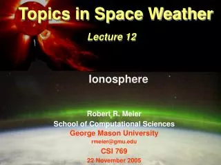
Topics in Space Weather Lecture 11 The Upper Atmosphere. Robert R. Meier School of Computational Sciences George Mason University rmeier@gmu.edu CSI 769 15 November 2005. Remaining Lectures. Lecture 11 – November 15 Upper Atmosphere Lecture 12 – November 22 Ionosphere

E N D
Topics in Space WeatherLecture 11The Upper Atmosphere Robert R. Meier School of Computational Sciences George Mason University rmeier@gmu.edu CSI 769 15 November 2005
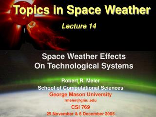
Remaining Lectures • Lecture 11 – November 15 • Upper Atmosphere • Lecture 12 – November 22 • Ionosphere • Geomagnetic storms • Lecture 13 – November 29 • Geomagnetic storms & magnetosphere connection • Aurora and Airglow • Lecture 14 – December 6 • Effects on Technological Systems • John Goodman will give last lecture
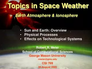
Topics - Lecture 11 • Sun as a star • Solar effects on the atmosphere • Upper atmospheric processes • Temperature • Density and composition • Winds
Sun-Earth System:Energy Coupling SUN EARTH convection zone radiative zone core particles and magnetic fields photons bow shock surface surface solar wind sunspot atmosphere atmosphere plage plasmasphere heliosphere coronal mass ejection magnetosphere not to scale
SOLAR - TERRESTRIAL ENERGY SOURCES Source Energy Solar Cycle Deposition (Wm-2) Change (Wm-2) Altitude • Solar Radiation • total 1366 1.2 surface • UV 200-300 nm 15.4 0.17 10-80 km • VUV 0-200 nm 0.15 0.15 50-500 km • Particles • electron aurora III 0.06 90-120 km • solar protons 0.002 30-90 km • galactic cosmic rays 0.0000007 0-90 km • Peak Joule Heating (strong storm) • E=180 mVm-1 0.4 90-200 km Solar Wind0.0006 above 500 km
TOTAL IRRADIANCE VARIABILITY SPECTRUM VARIABILITY
The Sun’s Radiation Spectrum UV radiation varies more than visible radiation because UV faculae are brighter sunspot faculae magnetic fields have different effects on radiation at different wavelengths
EUV Radiation is Emitted from the Sun’s Outer Atmosphere: Chromosphere, Corona He+ 304 EUV spectrum: >1500 lines 5 continua 304Å 0.08MK quiet Sun Warren et al., 2001 quiet Sun emission line temperatures vary over 2 orders of magnitude 19960304 20000502 EIT 284Å 2MK GOES 750K Exospheric Temperature 1300K flares and 27-day rotations superimposed on 11-year cycles
SOLAR IRRADIANCE VARIABILITY MECHANISMS SOLAR ACTIVITY CYCLE SOLAR ROTATION
Sun and Thermosphere-Ionosphere NRLMSIS:500 km quiet Sun solar EUV photon energy response to EUV photons response to particles, plasma, fields Ap solar wind kinetic energy NAVSPACECOM solar wind energy temperature corona spacecraft drag neutral density 16 JAN 03 electron density 400 km critical frequency chromosphere heliosphere nemax=1.24×10⁴fo2
EUV Radiation is Emitted from the Sun’s Outer Atmosphere: Chromosphere, Corona 304 EUV spectrum: >1500 lines 5 continua 304Å 0.08MK quiet Sun 19960304 EIT 20000502 quiet Sun emission line temperatures vary over 2 orders of magnitude 284Å 2MK 750K Exospheric Temperature 1300K Primary EUV Sources of Upper Atmosphere Heating: ch chromospheric cr coronal ch+cr mixed Roble, 1987
He II “304” Å Irradiance Variability 11-year cycle SOHO/ 27-day rotation model TIMED/ episodic flaring Solar Cycle EUV Spectrum Variability SEM “304”Å 5 min irradiance NRLEUVHFG EUVAC SOLAR2000 particle contamination
Solar EUV Radiation Alters Ionosphere - Bastille Day 2000 solar eruption SOHO EIT 195Å X-ray and EUV irradiance variation pre-flare ionospheric electron density response flare NRL SAMI2 model (Huber and Joyce) Meier et al., GRL, 2001 TRACE
Availability of Solar XR, EUV & UV Data • Solar Extreme Ultraviolet (SEE) data from NASA/TIMED satellite • http://lasp.colorado.edu/see/ • Solar Radiation and Climate Experiment (SORCE) • http://lasp.colorado.edu/sorce/ • Solar EUV model (EUV81) [Hinteregger et al., Geophys. Res. Lett. 8, 1147-1150, 1981] • Can be found at SEE website, along with other models (click on Data-General information and other data-Solar Irradiance Models)
Solar Energy Deposition Atmospheric Structure SPACE WEATHER GLOBAL CHANGE EUV FUV MUV RADIATION
Radiative energy deposition follows Beer’s Law F Change in solar flux n = # absorbers/cc • = absorption cross section Integrating, dz’ F+dF
Optical Depth • Definition • For several species • i = N2, O2, O • Altitude of unit optical depth: F(z)= F() e-1 • Solve (z) = 1 for z (See slide 16)
Column Density • If const., • Vertical Column Density number of atoms/molecules in a 1 cm2 column above altitude z
Assume plane parallel atmosphere H << earth radius Away from terminator s = z / cos and (s) = (z) / cos solar zenith angle What happens at the terminator ( = 90o)? Slant path optical depth F() 0 (s) s (z) z
Large solar zenith angles • Allowing for earth curvature and isothermal atmosphere, then: (s) = (z) Ch(x, ) • X = (Re + z)/H • Re = earth radius • H = scale height • Ch(x, ) = Chapman function where + > 90o and - < 90o • Must do numerical integration along slant path from Sun: • If not isothermal • If accounting for oblate spheroid shape of Earth * * From Rishbeth and Garriott, Intro. To Iono. Phys.
Solar Energy in the Upper Atmosphere ENERGETIC SUNLIGHT AND PARTICLES IONIZATION DISSOCIATION EXCITATION NEUTRAL CHEMISTRY ION CHEMISTRY COLLISIONAL DEACTIVATION PHOTOELECTRONS SPECTRAL EMISSIONS ELECTRON HEATING ION HEATING NEUTRAL HEATING
Atmospheric Absorption Processes • Ionization • O2 + h O2+ + e*, … • Dissociation • N2 + h N + N, … • Excitation • O + h O* • O* O + h ’ radiation • O* + X O + X quenching or deactivation • Dissociative ionization – excitation • N2 + h N+* + N + e, … . . .
Energy Thresholds for Processes* * From Heubner et al., Astrophys. Space Sci., 195, 1-294, 1992 Useful relationship: E(eV) x (Å) = 12397
N2 Absorption Cross Section * * Pl. Space Sci. 31, 597, 1983
O2 Absorption Cross Section * * Pl. Space Sci. 31, 597, 1983
SOLAR CYCLE CHANGES IN EUV RADIATION IMPACT UPPER ATMOSPHERE TEMPERATURE and DENSITY Solar Cycle Changes at 700 km: Neutral Temperature: 2 times Neutral Density: 50 times Electron Density: 10 times
Atmospheric Processes Described by Thermospheric Global Circulation Models (GCMs)
GCM Physics: Upper Atmosphere Geoff Crowley Atmospheric & Space Technology Research Associates (ASTRA) 11118 Quail Pass San Antonio, TX 78249 210-691-0432 Objective: What’s required to build a GCM? (Equations, numerical techniques, parameterizations, boundary conditions, input specifications, validation with data)
Important Inputs to the Thermosphere – Ionosphere System Solar UV Input E-fields Particles? Neutral density temperature wind electron density Upper Atmosphere (Thermosphere – Ionosphere) Tides and Gravity Waves
Tides Temperature Gravity Waves Winds E-fields Composition Electron Density Simplified Physics of Upper Atmosphere Joule Heating Particle Heating Solar EUV Chemical Heating Boundary Conds Diffusion Coeffs Chemistry Solar EUV
Molecular conduction radiation advection adiab. heating Many terms Energy equation The leap-frog method is employed with vertical thermal conductivity treated implicitly to second order accuracy. This leads to a tridiagonal scheme requiring boundary conditions at the top and bottom of the domain as implied by the differential equation. Advection is treated implicitly to fourth order in the horizontal, second order in the vertical
Vert. adv. Recombination Production molecular diffusion eddy diffusion Horiz. advection Continuity equation i is the mass mixing ratio for species i: i = I(z) / I(z), where is the mass density The leap-frog method is employed leading to a tridiagonal scheme requiring boundary conditions at the top and bottom of the domain.
Example: Nitrogen Chemistry (Simplified) Each species equation includes horizontal and vertical advection, photo-chemical production and loss, and vertical molecular and eddy diffusion.
Neutral Species The model includes 15 separate neutral species, not counting some excited states which are also tracked. CO2, O, N2, CO, O2, O3, H, H2, H2O, HO2, N, NO, NO2, Ar, and He. Ionized Species The model includes 7 ion species O+, N+, CO2+, O2+, N2+, NO+, and H+ with ionization primarily from solar EUV and x-ray. The ions are assumed to be in photochemical equilibrium with one another and the free electrons.
Momentum equations Zonal velocity Rayleigh friction Pressure gradients Coriolis gravity wave drag ion drag momentum advection Viscosity (Molecular and Eddy) Meridional velocity The Leap frog method is employed with vertical molecular viscosity treated implicitly to second order accuracy. Since the zonal and meridional momentum equations are coupled through Coriolis and off-diagonal ion drag terms, the system reduces to a diagonal block matrix scheme, where (2 x 2) matrices and two component vectors are used at each level. Boundary conditions for the zonal (u) and meridional ( v) wind components are needed at the top and bottom of the model.
Upper atmospheric temperature, density and composition Some simplified concepts
78% N2 21% O2 1% other
Thermodynamics • Temperature equation very difficult to solve • Even under simplified 1-D geometry, the temperature equation is a 2nd order time-dependent PDE • See Equation 8.77 of Gombosi • Net heating rate (Production – Loss) is positive in the thermosphere (low cooling rate) • Leads to increase in temperature with altitude • Heat conducted downward and radiated to space in the lower thermosphere by CO2, NO, and small amount of O fine structure radiation
Bates [1959] Temperature Profile Analytic approximation for temperature profile: T(z) = T - (T - Tzo) e-s(z – zo) • s = shape function • Varies with conditions • typical ~ 0.02 km-1 • Matches observations • Functional form agrees with GCM models
Fitting Bates Temperature Profile to GCM Model Low solar activity • Non-linear least squares fit • “+” are model • Lines are function • Worst error: few % • Therefore, can use Bates profile for simple models of the thermosphere • Note • Some places, T ~ const. • Some places, T ~ linear High solar activity
Diffusion • Eddy diffusion • Turbulent mixing/wave breaking approximated by diffusion of small eddys • Molecular diffusion • Each species follows its own scale height • Turbopause • Where eddy and molecular diffusion rates are equal • Typically ~ 105 km • But transition is smooth over some altitude interval • Below is called the homosphere • Above is the heterosphere
Turbopause Heterosphere Turbopause Homosphere Gombosi, Fig 8.3
Diffusive Equilibrium • Maxwell-Boltzmann velocity distribution • No net vertical diffusion velocity • No chemistry • Steady-state, static equilibrium • Ignore velocities • Chapter 8 [Gombosi]
(p+dp)A Diffusive Equilibrium Area A dz The Gibbs-Dalton Law of partial pressures applies. For any species, force balance yields: dw + (p+dp)A = pA but dw = g A dz Then dp = - g dz= - nm g dz where p = pressure = mass density n = molecules cm-3 m = molecular mass g = grav. acceleration dw z pA zo Forces balance on slab of gas in equilibrium at altitude z
Combine with Ideal Gas Law p = n k T dp = kT dn + nk dT = - nm g dz dividing by nkT dn/n + dT/T + dz/H = 0 where H = kT/(mg) If T and g constant, then n(z) = n(zo) e-(z-zo)/H Note-Earth is an oblate spheroid: • Equatorial Radius: 6378 km & g = 9.78 m/s2 • Polar Radius: 6357 km & g = 9.83 m/s2 • Mean Radius: 6371 km