Presentation on Probability Distribution * Binomial * Chi-square
Presentation on Probability Distribution * Binomial * Chi-square. Presenters: Nouruddin Boojhawoonah & Poonam Gopaul Notes reffered from statistics tutorial: Probability distribution. J.CRAWSHAW and J.CHAMBERS.


Presentation on Probability Distribution * Binomial * Chi-square
E N D
Presentation Transcript
Presentation on Probability Distribution* Binomial* Chi-square Presenters: NouruddinBoojhawoonah & PoonamGopaul Notes reffered from statistics tutorial: Probability distribution. J.CRAWSHAW and J.CHAMBERS
To understand probability distributions, it is important to understand variables. random variables, and some notation. • A variable is a symbol (A, B, x, y, etc.) that can take on any of a specified set of values. • When the value of a variable is the outcome of a statistical experiment, that variable is a random variable. Generally, statisticians use a capital letter to represent a random variable and a lower-case letter, to represent one of its values. For example, • X represents the random variable X. • P(X) represents the probability of X. • P(X = x) refers to the probability that the random variable X is equal to a particular value, denoted by x. As an example, P(X = 1) refers to the probability that the random variable X is equal to 1.
Probability Distributions An example will make clear the relationship between random variables and probability distributions. Suppose you flip a coin two times. This simple statistical experiment can have four possible outcomes: HH, HT, TH, and TT. Now, let the variable X represent the number of Heads that result from this experiment. The variable X can take on the values 0, 1, or 2. In this example, X is a random variable; because its value is determined by the outcome of a statistical experiment. A probability distribution is a table or an equation that links each outcome of a statistical experiment with its probability of occurence. Consider the coin flip experiment described above. The table below, which associates each outcome with its probability, is an example of a probability distribution. The below table represents the probability distribution of the random variable X.
Cumulative Probability Distributions A cumulative probability refers to the probability that the value of a random variable falls within a specified range. Let us return to the coin flip experiment. If we flip a coin two times, we might ask: What is the probability that the coin flips would result in one or fewer heads? The answer would be a cumulative probability. It would be the probability that the coin flip experiment results in zero heads plus the probability that the experiment results in one head. P(X < 1) = P(X = 0) + P(X = 1) = 0.25 + 0.50 = 0.75 Like a probability distribution, a cumulative probability distribution can be represented by a table or an equation. In the table below, the cumulative probability refers to the probability than the random variable X is less than or equal to x.
Uniform Probability Distribution The simplest probability distribution occurs when all of the values of a random variable occur with equal probability. This probability distribution is called the uniform distribution. Uniform Distribution. Suppose the random variable X can assume k different values. Suppose also that the P(X = xk) is constant. Then, P(X = xk) = 1/k Example 1Suppose a die is tossed. What is the probability that the die will land on 6 ? Solution: When a die is tossed, there are 6 possible outcomes represented by: S = { 1, 2, 3, 4, 5, 6 }. Each possible outcome is a random variable (X), and each outcome is equally likely to occur. Thus, we have a uniform distribution. Therefore, the P(X = 6) = 1/6. Example 2Suppose we repeat the dice tossing experiment described in Example 1. This time, we ask what is the probability that the die will land on a number that is smaller than 5 ? Solution: When a die is tossed, there are 6 possible outcomes represented by: S = { 1, 2, 3, 4, 5, 6 }. Each possible outcome is equally likely to occur. Thus, we have a uniform distribution. This problem involves a cumulative probability. The probability that the die will land on a number smaller than 5 is equal to: P( X < 5 ) = P(X = 1) + P(X = 2) + P(X = 3) + P(X = 4) = 1/6 + 1/6 + 1/6 + 1/6 = 2/3
If a variable can take on any value between two specified values, it is called a continuous variable; otherwise, it is called a discrete variable. Some examples will clarify the difference between discrete and continuous variables. • Suppose the fire department mandates that all fire fighters must weigh between 150 and 250 pounds. The weight of a fire fighter would be an example of a continuous variable; since a fire fighter's weight could take on any value between 150 and 250 pounds. • Suppose we flip a coin and count the number of heads. The number of heads could be any integer value between 0 and plus infinity. However, it could not be any number between 0 and plus infinity. We could not, for example, get 2.5 heads. Therefore, the number of heads must be a discrete variable. Just like variables, probability distributions can be classified as discrete or continuous. Discrete Probability Distributions If a random variable is a discrete variable, its probability distribution is called a discrete probability distribution.
Binomial Distribution To understand binomial distributions and binomial probability, it helps to understand binomial experiments and some associated notation; so we cover those topics first. Binomial Experiment A binomial experiment (also known as a Bernoulli trial) is a statistical experiment that has the following properties: • The experiment consists of n repeated trials. • Each trial can result in just two possible outcomes. We call one of these outcomes a success and the other, a failure. • The probability of success, denoted by P, is the same on every trial. • The trials are independent; that is, the outcome on one trial does not affect the outcome on other trials. Consider the following statistical experiment. You flip a coin 2 times and count the number of times the coin lands on heads. This is a binomial experiment because: • The experiment consists of repeated trials. We flip a coin 2 times. • Each trial can result in just two possible outcomes - heads or tails. • The probability of success is constant - 0.5 on every trial. • The trials are independent; that is, getting heads on one trial does not affect whether we get heads on other trials. Notation The following notation is helpful, when we talk about binomial probability. • x: The number of successes that result from the binomial experiment. • n: The number of trials in the binomial experiment. • P: The probability of success on an individual trial. • Q: The probability of failure on an individual trial. (This is equal to 1 - P.) • b(x; n, P): Binomial probability - the probability that an n-trial binomial experiment results in exactlyx successes, when the probability of success on an individual trial is P. • nCr: The number of combinations of n things, taken r at a time.
Binomial Distribution A binomial random variable is the number of successes x in n repeated trials of a binomial experiment. The probability distribution of a binomial random variable is called a binomial distribution (also known as a Bernoulli distribution). Suppose we flip a coin two times and count the number of heads (successes). The binomial random variable is the number of heads, which can take on values of 0, 1, or 2. The binomial distribution is presented below. The binomial distribution has the following properties: • The mean of the distribution (μx) is equal to n * P . • The variance (σ2x) is n * P * ( 1 - P ). • The standard deviation (σx) is sqrt[ n * P * ( 1 - P ) ]. Binomial Probability The binomial probability refers to the probability that a binomial experiment results in exactlyx successes. For example, in the above table, we see that the binomial probability of getting exactly one head in two coin flips is 0.50. Given x, n, and P, we can compute the binomial probability based on the following formula: Binomial Formula. Suppose a binomial experiment consists of n trials and results in x successes. If the probability of success on an individual trial is P, then the binomial probability is: P(X=r)= (nCr).qn-r.pr
Lets work out an example30% of pupils in a school travel by bus. From a sample of ten pupils chosen at random, find the probability that(a) only three travel by bus,(b) less than half travel by busHints: (we need to identify n=? & p=?)
Other examples (1) The random variable X~Bin(6, .042). Find P(X= 6) P(X= 4) P(X≤ 2) (2) A fair coin is tossed six times. Find the probability of throwing at least four heads. (3) X~Bin(n, 0.3). Find the least possible value of n such that P(X≥1)= 0.8. (4) Assuming that a couple are equally likely to produce a boy or a girl, find the probability that in a family of five children there are more boys than girls.
(5) X~Bin(4, p) and P(X=4)= 0.0256. Find P(X=2). (6) Charlie finds that when she takes a cutting from a particular plant, the probability that it roots successfully is 1/3. She takes nine cuttings. Find the probability that (i) more than five cuttings root successfully, (ii) at least three cuttings root successfully, (b) Find the number of cuttings that she should take in order to be 99% certain that at least one cutting root successfully.
Example to illustrate Diagrammatic representation of the Binomial DistributionIn a survey on washing powder, it is found that the probability that a shopper chooses Soapsuds is 0.35. Using a sample of seven shoppers, illustrate the information in a diagram.Solution:X~Bin(7, 0.35)P(X=r) = (7Cr).qn-r.prP(X=0)= 0.0490P(X=1)= 0.1847P(X=2)= 0.2984P(X=3)= 0.2678P(X=4)= 0.1442P(X=5)= 0.0466P(X=6)= ???P(X=7)= ???
p X~Bin(7, 0.35) 0 X
Expectation and Variance of the Binomial Distribution If X~Bin(n, p) E(X)=np VAR(X)=npq, where q= 1-p Computation of Expectation and Variance for a probability distribution table E(X)= ExP(X=r) E(X^2)= Ex^2P(X=r) VAR(X)= E(X^2)-E^2(X)
The random variable X~Bin(4, 0.8). Construct the probability distribution for X and find the expectation and variance. Verify that E(X)= np and Var(X)= npq X~Bin(4,0.8) so n=4 and p=0.8 P(X=0)= 0.2^4 =0.0016 P(X=1) = 4*0.2^3*0.8 =0.0256 P(X=2)= 4C2*0.2^2*0.8^2 =0.1536 P(X=3)= 4C3*0.2*0.8^3 =0.4096 P(X=4)=0.8^4 =0.4096 Probability distribution table for X:
E(X)= ExP(X=r) = 0*0.0016 + 1*0.0256 + 2*0.1536 + 3*0.4096 + 4*0.4096 = 3.2 E(X^2)= Ex^2P(X=r) = (0^2*0.0016) + (1^2*0.0256) + (2^2*0.1536) + (3^2*0.4096) + (4^2*0.4096) = 10.88 VAR(X) = E(X^2)-E^2(X) = 10.88- (3.2^2) = 0.64 Now, np= 8*0.4 = 3.2 npq= 8*0.4*0.6 = 0.64 Therefore, E(X)= np VAR(X)= npq
THE X2TEST The X2 test is a significance test that enables us to decide whether it is valid to use a particular distribution, such as binomial,poissonor normal, as a model so that we can interpret observed data. We can also use the X2 test to decide Whether two variables are independent.
Example: • A farmer Kept a record of the number of heifer calves born to each of his cows during the first five years of breeding of each cow. The results are summarized below • Test, at 5% Level of significance, whether or not the binomial distribution with parameters n=5,p=0.5 is an adequate model for these distribution
procedures • Consider a set of data with observed frequency, O • Make the null hypothesis(ho ) concerning the distribution followed by the data. Let X be the r.v.’the number of heifer calves born to a cow in the first five years of breeding’. Ho:X~Bin(5,0.5) • Calculate the expected frequencies,E according to this hypothesis. The expected frequencies are given by 150p(X=x) where P(X=x)=5cx(o.5)5-x(o.5)x =5cx(0.5)5
)5 150x 5c0 (0.5)5 150x 5c1 (0.5)5 150 x 5c2 (0.5)5
Since the expected frequencies for the first and last cells are less than 5, We must combine them with the next cell. 4.7+23.4 4.7+23.4
Work out the number of degrees of freedom v Where v= Number of cells- Number of restrictions The Number of restriction depends on the null hypothesis The number of cells=4 There is one restriction, that the total expected frequency is150. Therefore, v =4-1=3 Decide on the level of the test and the rejection criterion, looking up the critical values in the x2 tables The x2(3) distribution is considered.
We test at the 5% level and reject H0 if x2> x25% (3),i.e. if x2>7.82
X2=Sum(O-E)2/E = 3.461 Since X2 <7.82, we do not reject Ho and we conclude that the binomial distribution with n=5 and p= 0.5 is an adequate model for the data
Thank you all for your kind attention, if ever there still any doubt left somewhere, do feel free to ask me after lecture session.