Understanding Shadow Prices and Reduced Costs in Linear Programming Constraints
This overview discusses the concepts of shadow prices and reduced costs in linear programming, differentiating between tight and slack constraints, as well as sign and nonnegativity constraints. Key interpretations regarding duality and how changes in objective functions and constraint capacities affect profitability and resource allocation are explored. The application of these concepts with real-world examples, such as recreational vehicle production, demonstrates the practical implications of linear models. Additionally, the methods for generating sensitivity reports using tools like Excel Solver are highlighted.

Understanding Shadow Prices and Reduced Costs in Linear Programming Constraints
E N D
Presentation Transcript
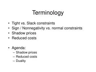
Terminology • Tight vs. Slack constraints • Sign / Nonnegativity vs. normal constraints • Shadow prices • Reduced costs • Agenda: • Shadow prices • Reduced costs • Duality
Shadow Prices • (Change in objective) / (Change in constraint right hand side) • 0 for loose constraints • Applies to normal constraints • Interpretation: • Price for additional capacity
Reduced Cost • Shadow price for x >= 0 constraints • 0 for variables that are positive • Change in objective when variable set to 1 • Making constraint tighter • Objective becomes worse • Contribution (profit from setting variable to 1) - opportunity cost (loss from reallocating resources)
Recreational Vehicles Example • Shadow prices: • E (engine shop) = $140/hr • B (body shop) = $420/hr • Reduced cost for L (luxury car) • Contribution $1200 • Opportunity cost,needs 1hr in engine shop + 3hr in body shop= 1E+3B=$1400 • Reduced cost = 1200-1400= $ -200
Excel • Solver -> options -> “assume linear model” • Solver -> Solve -> Sensitivity Report • Concepts apply to nonlinear problems too • Shadow price = “Lagrange multiplier” • Reduced cost = “Reduced gradient”
Dual Problem • Theory is works particularly for LPs • Also an LP (when original is an LP) • Another way of understanding problem • Normal constraints become variables • Variables become constraints • Max becomes min • …
Dual Problem Dual: min cost to buy all capacity s.t. willing to sell capacity instead of produce variables are prices Original: max profit from running plant s.t. capacity not exceeded variables are production quantities
Dual Problem Dual: min price E * 120 hr engine shop capacity + … s.t. 3hr * E + 1hr *B + 2hr * SF >= $840 (car profit) … variables E, B, SF, FF, FL are prices Original: max $840 profit * S cars + … s.t. 3hr * S + 2hr * F + 1hr * L <= 120hr engine shop capacity … variables S, F, L are production quantities
Dual Problem maxx pTx s.t. Ax <= c x >= 0 equivalent to miny cTy s.t. ATy >= p y >= 0