Trees Featuring Minimum Spanning Trees

1. TreesFeaturing Minimum Spanning Trees HKOI Training 2005 Advanced Group Presented by Liu Chi Man (cx)

2. Prerequisites • Asymptotic complexity • Set theory • Elementary graph theory • Priority queues

3. Assumptions • In the coming slides, we only talk about simple graphs • Extensions to multigraphs and pseudographs should be straightforward if you understand the materials well

4. Notations • A graph G = (V, E) • V is the set of vertices • E is the set of edges • |V| is the number of vertices in V • Sometimes we use V for convenience • |E| is the number of edges in E • Sometimes we use E for convenience

5. Uh… a long way to go • What is a Tree? • Disjoint Sets • Minimum Spanning Trees • Various Tree Topics

6. What is a Tree? A tree in Pokfulam, Hong Kong. (Photographer: cx)

7. What is a Tree? • In graph theory, a tree is an acyclic, connected graph • Acyclic means “with no cycles”

8. What is a Tree? • Properties of a tree: • |E| = |V| - 1 • |E| = (|V|) • Adding an edge between a pair of non-adjacent vertices creates exactly one cycle • Removing any one edge from the tree makes it disconnected

9. What is a Tree? • The following four conditions are equivalent: • G is connected and acyclic • G is connected and |E| = |V| - 1 • G is acyclic and |E| = |V| - 1 • Between any pair of vertices in G, there exists a unique path • G is a tree if at least one of the above conditions is satisfied

10. Other Properties of Trees • A tree is bipartite • A tree with at least two vertices has at least two leaves (vertices of degree 1) • A tree is planar

11. ZzZZzzz… bored to death? • What is a Tree? • Disjoint Sets • Minimum Spanning Trees • Various Tree Topics

12. The Union-Find Problem • Initially there are N objects, each in its own singleton set • Let’s label the objects by 1, 2, …, N • So the sets are {1}, {2}, …, {N} • There are two kinds of operations: • Merge two sets (Union) • Find the set to which an object belongs • Let there be a sequence of M operations

13. The Union-Find Problem • An example, with N = 4, M = 5 • Initial: {1}, {2}, {3}, {4} • Union {1}, {3} {1, 3}, {2}, {4} • Find 3. Answer: {1, 3} • Union {4}, {1,3} {1, 3, 4}, {2} • Find 2. Answer: {2} • Find 1. Answer {1, 3, 4}

14. Disjoint Sets • We usually use disjoint-set data structures to solve the union-find problem • A disjoint set is simply a data structure that supports the Union and Find operations • How should a set be named? • Each set has its own representative element

15. Disjoint Sets • Implementation: Naïve arrays • Set[x] stores the representative of the set containing x, for 1 ≤ x ≤ N • <per Union, per Find>: <O(N), O(1)> • Slight modifications give <O(U), O(1)> • U is the size of the union • Worst case is O(MN) for all M operations

16. Disjoint Sets • An example, with N = 4 Initial: Union 1 3: Union 2 4: Answer = 2 Find 4: Union 1 2: Answer = 1 Find 4:

17. Disjoint Sets • Why is it slow? • Consider Union 1 2 on the table:

18. Disjoint Sets • Idea for improvement: • When doing a Union, always update the set of smaller size • The overall running time can be shown to be O(M lgN)

19. 6 1 3 5 4 7 2 Disjoint Sets • Implementation: Forest • A forest is a set of trees • Each set is represented by a rooted tree, with the root being the representative element Two sets: {1, 3, 5} and {2, 4, 6, 7}.

20. Disjoint Sets • Ideas • Find • Traverses from the vertex up to the root • Union • Merges two trees in the forest • That is, the root of one tree becomes a child of the other tree

21. 1 2 3 4 1 2 4 3 1 2 3 4 1 2 3 4 Disjoint Sets • An example, with N = 4 Initial: Union 1 3: Union 2 4: Find 4:

22. 1 2 3 4 1 2 3 4 Disjoint Sets • An example, with N = 4 (cont.) Union 1 2: Find 4:

23. Disjoint Sets • How to represent the trees? • Leftmost-Child-Right-Sibling (LCRS)? • Too complex! • We just need to traverse from bottom to top – parent-finding should be supported • An array Parent[] is enough • Parent[x] stores the parent vertex of x if x is not the root of a tree • Parent[x] stores x if x is the root of a tree

24. Disjoint Sets • The worst case is still O(MN ) overall • To improve the worst case time complexity, we employ two techniques • Union-by-rank • Path compression

25. Disjoint Sets • Union-by-rank • Recall that in our previous naïve array implementation, the worst case time bound can be improved by always updating the smaller set in a Union • Here, we make the “smaller” tree a subtree of the “larger” tree • To keep the resulting tree “small” • To compare the “sizes” of trees, we assign a rank to every tree in the forest

26. Disjoint Sets • Union-by-rank (cont.) • The rank of the tree is the height of the tree when it is created • A tree is created either at the beginning, or after a Union • That means we need to keep track of the trees’ ranks during the Unions

27. Disjoint Sets • Path compression • See also the solution for Symbolic Links (HKOI2005 Senior Final) • When we carry out a Find, we traverse from a vertex to the root • Why don’t we move the vertices closer to the root at the same time? • Closer to the root means shorter query time

28. The root is 3 3 3 3 5 5 1 5 1 6 1 4 6 6 The root is 3 7 2 4 4 The root is 3 7 7 2 2 Disjoint Sets • An example, with N = 7 • Now we Find 4

29. Disjoint Sets • We ignore the effect of path compression on tree ranks • Union-by-rank alone gives a running time of O(M lgN) • Together with path compression, the improved running time is O(M(N)) •  is the inverse of the Ackermann's function • (n) is almost constant

30. When can I have my lunch? • What is a Tree? • Disjoint Sets • Minimum Spanning Trees • Various Tree Topics

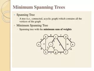
31. Minimum Spanning Trees • Given a connected graph G = (V, E), a spanning tree of G is a graph T such that • T is a subgraph of G • T is a tree • T contains every vertex of G • A connected graph must have at least one spanning tree

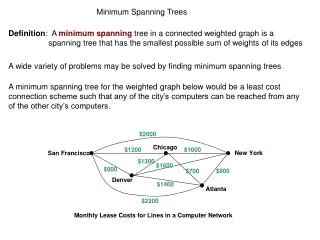
32. Minimum Spanning Trees • Given a weighted connected graph G, a minimum spanning tree T* of G is a spanning tree of G with minimum total edge weight • Application: Minimizing the total length of wires needed to connect up a collection of computers

33. Minimum Spanning Trees • Two algorithms • Kruskal’s algorithm • Prim’s algorithm

34. Kruskal’s Algorithm • Algorithm • Initially T is an empty set • While T has less than |V|-1 edges Do • Choose an edge with minimum weight such that it does not form a cycle with the edges in T, and add it to T • The edges in T form a MST

35. Kruskal’s Algorithm • Algorithm (Detailed) • T is an empty set • Sort the edges in G by their weights • For (in ascending weight) each edge e Do • If T  {e} does not contain a cycle Then • Add e to T • Return T

36. Kruskal’s Algorithm • How to check if a cycle is formed? • Depth-first search (DFS) • Time complexity is O(E2) • Alternatively, a disjoint set! • The sets are connected components

37. Kruskal’s Algorithm • Algorithm (disjoint-set) • T is an empty set • Create sets {1}, {2}, …, {V} • Sort the edges in G by their weights • For (in ascending weight) each edge e Do • Let e connect vertices x and y • If Find(x)  Find(y) Then • Add e to T, then Union(Find(x), Find(y)) • Return T

38. Kruskal’s Algorithm • The improved time complexity is O(ElgV) • In fact, the bottleneck is sorting!

39. Prim’s Algorithm • Algorithm • Initially T is a set containing any one vertex in V • While T has less than |V|-1 edges Do • Among those edges connecting a vertex in T and a vertex in V-T, choose one with minimum weight, and add it (with its two end vertices) to T • T is a minimum spanning tree

40. Prim’s Algorithm • Algorithm (Detailed) • T   • Cost[x]  for all x  V • Marked[x]  false for all x  V • Pred[x]   for all x  V • Pick any u V, and set Cost[u] to 0 • Repeat |V| times • Let w be a vertex of minimum Cost among all unMarked vertices • Marked[w]  true • T  T  Pred[x] • For each unMarked vertex v such that (w, v)  E Do • If weight(w, v) < Cost[v] Then • Cost[v]  weight(w, v) • Pred[x]  { (w, v) } • Return T

41. Prim’s Algorithm • Time complexity: O(V2) • If a (binary) heap is used to accelerate the Find-Min operations, the time complexity is reduced to O(ElgV) • O(VlgV+E) if a Fibonacci heap is used

42. Minimum Spanning Trees • The fastest known algorithm runs in O(E(V,E))

43. MST Extensions • Second-best MST • We don’t want the best! • Online MST • See IOI2003 Path Maintenance • Minimum Bottleneck Spanning Tree • The bottleneck of a spanning tree is the weight of its maximum weight edge • An algorithm that runs in O(V+E) exists

44. MST Extensions (NP-Hard) • Minimum Steiner Tree • No need to connect all vertices, but at least a given subset B  V • Degree-bounded MST • Every vertex of the spanning tree must have degree not greater than a given value K

45. Are you with me? • What is a Tree? • Disjoint Sets • Minimum Spanning Trees • Various Tree Topics

46. Various Tree Topics • Center and diameter • Tree isomorphism • Canonical representation • Prüfer code • Lowest common ancestor (LCA)

47. Supplementary Readings • Advanced: • Disjoint set forest (Lecture slides) • Prim’s algorithm • Kruskal’s algorithm • Center and diameter • Post-advanced (so-called Beginners): • Lowest common ancestor • Maximum branching