Advanced Nonlinear Programming Models for Optimization Education
Explore general formulations, solution characteristics, convexity, and examples in nonlinear optimization. Learn to differentiate local vs. global solutions and grasp the complexities of real-world engineering problems.

Advanced Nonlinear Programming Models for Optimization Education
E N D
Presentation Transcript
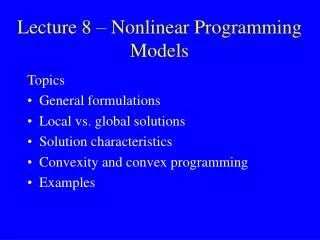
Lecture 8 – Nonlinear Programming Models Topics • General formulations • Local vs. global solutions • Solution characteristics • Convexity and convex programming • Examples
Nonlinear Optimization • In LP ... the objective function & constraints are linear and the problems are “easy”to solve. • Many real-world engineering and business problems have nonlinear elements and are hard to solve.
General NLP Minimize f(x) s.t. gi(x) (, , =) bi, i = 1,…,m x = (x1,…,xn) is the n-dimensional vector of decision variables f(x) is the objective function gi(x) are the constraint functions bi are fixed known constants
… c x c x c x Example 2 Max f(x) = e e e 1 1 2 2 n n s.t. Ax = b, x³0 n å fj (xj) Example 3 Min Problems with “decreasing efficiencies” j =1 s.t. Ax = b, x³0 fj(xj) where each fj(xj)is of the form xj Examples of NLPs 4 Example 1 Max f(x) = 3x1 + 2x2 2 s.t. x1 + x2£ 1, x1³ 0, x2 unrestricted Examples 2 and 3 can be reformulated as LPs
NLP Graphical Solution Method Max f(x1, x2) = x1x2 s.t. 4x1 + x2£ 8 x1 ³ 0, x2 ³ 0 x2 8 f(x) = 2 f(x) = 1 x1 2 Optimal solution will lie on the line g(x) = 4x1 + x2 – 8 = 0.
Solution Characteristics Gradient of f(x) = f(x1, x2) (f/x1, f/x2)T This gives f/x1 = x2, f/x2 = x1 and g/x1 = 4, g/x2 = 1 At optimality we have f(x1, x2) = g(x1, x2) or x1* = 1 and x2* = 4 • Solution is not a vertex of feasible region. For this particular problem the solution is on the boundary of the feasible region. This is not always the case. • In a more general case, f(x1, x2) = g(x1, x2) with 0. (In this case, = 1.)
Nonconvex Function global max stationary point f(x) local max local min local min x Let Sn be the set of feasible solutions to an NLP. Definition: A global minimum is any x0S such than f(x0) f(x) for all feasible x not equal to x0.
Function with Unique Global Minimum at x = (1, –3) If g1 = x1³ 0 and g2 = x2³ 0, what is the optimum ? At (1, 0), f(x1, x2) = 1g1(x1, x2) + 2g1(x1, x2) or (0, 6) = 1(1, 0) + 2(0, 1), 1³ 0, 2³ 0 so 1 = 0 and 2 = 6
Function with Multiple Maxima and Minima Min { f(x)= sin(x) : 0 x 5p}
Constrained Function with Unique Global Maximum and Unique Global Minimum
f (x) Convexity condition for univariate f : d2 f(x) ≥ 0 for all x dx2 x1 x2 Convexity Convex function: If you draw a straight line between any two points on f(x) the line will be above or on f(x). Concave function: If f(x) is convex than –f(x) is concave. Linear functions are both convex and concave.
Definition of Convexity Let x1 and x2 be two points (vectors) in Sn. A function f(x) is convex if and only if f(lx1 + (1–l)x2) ≤ lf(x1) + (1–l)f(x2) for all 0 < l < 1. It is strictly convex if the inequality sign ≤ is replaced with the sign <. 1-dimensional example
Nonconvex -- Nonconave Function f(x) x x1 x2
2 2 2 d f d f d f Hessian of f at x : s2f(x) = . . . dx dx dx dx 2 dx 1 2 1 n 1 . . 2 d f . . . dx dx . 2 1 . . . 2 2 d f d f . . . dx dx 2 dx n 1 n Theoretical Result for Convex Functions A positively weighted sum of convex functions is convex: If fk(x) is convex for k =1,…,m and 1,…,m³ 0, then f(x) = å ak fk(x) is convex. m k =1 Used to determine convexity.
f(x) x1 x2 Determining Convexity One-Dimensional Functions: A function f(x) ÎC1 is convex if and only if it is underestimated by linear extrapolation; i.e., f(x2) ≥ f(x1) + (df(x1)/dx)(x2 – x1) for all x1 and x2. A function f(x) C2 is convex if and only if its second derivative is nonnegative. d2f(x)/dx2≥ 0 for all x If the inequality is strict (>), then f(x) is strictly convex.
Example: f(x) = 3(x1)2 + 4(x2)3 – 5x1x2 + 4x1 Multiple Dimensional Functions f(x) is convex if only if f(x2) ≥ f(x1) + Tf(x1)(x2 – x1) for all x1 and x2. Definition: The Hessian matrix H(x) associated with f(x) is the nn symmetric matrix of second partial derivatives of f(x) with respect to the components of x. When f(x) is quadratic, H(x) has only constant terms; when f(x) is linear, H(x) does not exist.
Properties of the Hessian How can we use Hessian to determine whether or not f(x) is convex? • H(x) is positive definite if and only if xTHx> 0 for all x0. • H(x) is positive semi-definite if and only if xTHx≥ 0 for all x and there exists and x 0 such that xTHx = 0. • H(x) is indefinite if and only if xTHx> 0 for some x, and xTHx< 0 for some other x.
Multiple Dimensional Functions and Convexity • f(x) is strictly convex (or just convex) if its associated Hessian matrix H(x) is positive definite (semi-definite) for all x. • f(x) is neither convex nor concave if its associated Hessian matrix H(x) is indefinite The terms negativedefiniteandnegative-semi- definiteare also appropriate for the Hessian and provide symmetric results for concave functions. Recall that a function f(x) is concave if –f(x) is convex.
Definition: The ith leading principal submatrix of H is the matrix formed taking the intersection of its first i rows and i columns. Let Hi be the value of the corresponding determinant: Testing for Definiteness , where hij= 2f(x)/xixj LetHessian, H =
Rules for Definiteness • H is positive definite if and only if the determinants of all the leading principal submatrices are positive; i.e., Hi> 0 for i = 1,…,n. • His negative definite if and only if H1 < 0 and the remaining leading principal determinants alternate in sign: • H2 > 0, H3 < 0, H4 > 0, . . . Positive-semidefinite and negative semi-definiteness require that all principal submatrices satisfy the above conditions for the particular case.
Quadratic Functions Example 1: f(x) = 3x1x2 + x12 + 3x22 so H1 = 2 and H2 = 12 – 9 = 3 Conclusion f(x) is convex because H(x) is positive definite.
Quadratic Functions (cont’d) Example 2: f(x) = 24x1x2 + 9x12 + 16x22 • so H1 = 18 and H2 = 576 – 576 = 0 • Thus H is positive semi-definite (determinants of all submatrices are nonnegative) so f(x) is convex. • Note, xTHx = 2(3x1 + 4x2)2≥ 0. For x1 = -4, x2 = 3, we get xTHx = 0.
Nonquadratic Functions Example 3: f(x) = (x2 – x12)2 + (1 – x1)2 Thus the Hessian depends on the point under consideration: At x = (1, 1), which is positive definite. At x = (0, 1), which is indefinite. Thus f(x) is not convex although it is strictly convex near (1, 1).
What You Should Know About Nonlinear Programming • How to develop models with nonlinear functions. • The definition of convexity. • Rules for positive and negative definiteness • How to identify a convex function. • The difference between a local and global solution.

