Computational Statistics with Application to Bioinformatics
170 likes | 249 Vues
Understand qualitative and quantitative tree models for biological classification using hierarchical clustering methods. Explore the benefits and limitations of additive trees and the efficiency of the Neighbor Joining algorithm in recovering phylogenetic relationships. Discover the application of these techniques in gene expression data analysis and biological research.

Computational Statistics with Application to Bioinformatics
E N D
Presentation Transcript
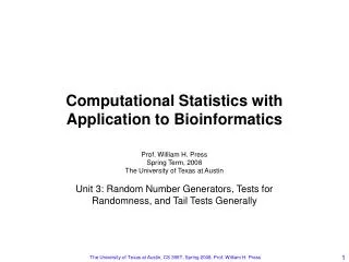
Computational Statistics withApplication to Bioinformatics Prof. William H. PressSpring Term, 2008The University of Texas at Austin Unit 10: Hierarchical Clustering by Phylogenetic Trees The University of Texas at Austin, CS 395T, Spring 2008, Prof. William H. Press
Compare qualitative and quantitative trees qualitative trees (“cladograms” or “fully parenthesized expressions”) don’t have a distance measure quantitative trees (e.g., additive trees or ultrametric trees) do additive tree much more restricted representation than general distance matrix If a distance matrix comes from an additive tree, there is an efficient O(N2) method for recovering the tree “Neighbor Joining” (NJ) And, it gives reasonably good approximate answers to the NP problem of what is the closest tree to a distance matrix Neighbor Joining is one example of the general agglomerative method Other agglomerative methods (e.g., WPGMA) are exact for ultrametric trees Ultrametric trees once thought important in biology, now not so Example: We recover a pretty good phylogeny of the vertebrates from a random ~128 base pairs in the genome use Hamming distance NJ trees are intrinsically unrooted – get root from other information Example: Clustering of genes by their co-expression in gene expression data Pearson r correlation gives distance matrix Unit 10: Hierarchical Clustering by Phylogenetic Trees (Summary) The University of Texas at Austin, CS 395T, Spring 2008, Prof. William H. Press
Classification by Phylogenetic Trees This is more general than just biology. Useful any time that you want do discover or visualize “closeness” relationships. Can be qualitative (groupings, no distances): Note that binary tree is general case if allow zero distances Or quantitative (a tree model for distances): The University of Texas at Austin, CS 395T, Spring 2008, Prof. William H. Press
d d N N n o n e o s e s 0 1 d d d 0 ( ) = ¢ ¢ ¢ b h l d h N N N i 2 2 1 2 t t ¡ ¡ 0 1 0 2 0 3 r a n c e n s g a n s c e s d d d 0 ¢ ¢ ¢ 0 1 1 2 1 3 B C B C d d d 0 ¢ ¢ ¢ 0 2 1 2 2 3 @ A ¢ ¢ ¢ Note that the tree model is a much more restricted representation than a general distance matrix. “additive tree” (prove by induction) distance matrix The University of Texas at Austin, CS 395T, Spring 2008, Prof. William H. Press
Can get distance matrix from tree not amazing Can test whether a distance matrix came from an additive tree the four point test slightly amazing, but O(N4) There is an efficient O(N2) algorithm for actually constructing the tree neighbor joining (NJ) also reduces the four point test to O(N2) amazing! Applied to distance matrices that are not additive trees, NJ produces a good approximation to the closest additive tree which is often itself a remarkably good approximation to the full distance matrix really amazing since the exact problem is known to be NP not completely understood! Facts (some amazing) about additive trees Four point test:For all distinct i,j,k,l there is at least one tie among the three sums of the form dij+dkl above: [eg]+[fh] = [eh]+[fg]can you see why this always works? The University of Texas at Austin, CS 395T, Spring 2008, Prof. William H. Press
Initialize N active clusters with one leaf node in each Then repeat exactly N-2 times: find the two active clusters that are closest by some prescribed1 distance measure create a new active cluster that combines the two connect the new active cluster (parent) to the two (children) specify branch lengths by some prescription2 delete the two children from the active list compute by some prescription1 distances from the new cluster to the other clusters Several useful algorithms are “agglomerative methods” Different agglomerative methods differ only in the two1,2 prescriptions. NJ is an agglomerative method that is exact for additive trees. WPGMA is an agglomerative method that is exact for ultrametric trees. The University of Texas at Austin, CS 395T, Spring 2008, Prof. William H. Press
I downloaded a (literally) random piece of the human genome that has alignments to 21 other vertebrates hg18.chr1 1550026 128 + 247249719 CCCTCTTGCAGTGTCACACTGAGTCCC… panTro2.chr1 1550081 128 + 229974691 CCCTCTTGCAGTGTCACACTGAGTCCC… rheMac2.chr1 4687633 128 + 228252215 CCCTCTTGCAGTGTCACGCTGAGTCCC… tupBel1.scaffold_142366.1-9639 6335 128 - 9639 CTCTCTTGCAGTGTCACGCTGAGTCCC… eriEur1.scaffold_329849 4248 128 - 16173 CTTCCTTGTAGGGTGACGCTGAGCCCC… bosTau3.chr16 24854618 126 - 72834534 --TTCCCGTAGGGTCATGCTGAGTCCC… equCab1.chrUn 152279254 126 - 405909753 --CTTTTGCAGGGTAATGCTGAGTCCC… felCat3.scaffold_207897 9337 126 - 11103 --CTCTTGCAGGGTCACGCTGAGTCCC… canFam2.chr5 59689323 126 + 91976430 --TTCTTGCAGGGTCACGCTGAGTCCC… mm8.chr4 526108 126 - 155029701 --CTCTTACAGGGTTACGCTGAGCCCC… rn4.chr5 600229 126 - 173096209 --CTCTTACAGGGTTACGCTGAGTCCC… echTel1.scaffold_295407 3308 128 + 9723 CTCTCCTGCAGCATCACCCTGAGCCCC… monDom4.chr2 103757048 128 + 541556283 CTCTCTTGCAGAGTCACCGTGAGTGCC… ornAna1.Contig30834 338 126 - 8660 --CCCTTGCAGAGTCTCCGTGAGTCCC… anoCar1.scaffold_2684 12615 123 - 15861 CCTCCTTGCAGAGTTACTGTGAGTCCG… galGal3.chr21 4917466 120 - 6959642 ---TTTTTCAGAGTCCTAGTGAGTCCT… xenTro2.scaffold_414 492398 124 + 1070475 TTTTTGTGCAGAGTCATACTGAGCACT… fr2.chrUn 185937056 125 - 400509343 TGTCGTCACAGAGTGAGTTTGGCGCCG… tetNig1.chrUn_random 28277029 125 + 171761319 TCTCATCACAGAGTGAGTTTGGCGCCG… danRer4.chrNA_random 3175416 123 + 208014280 CTTCTTCTCAGGGTGAGTTTGACGCCG… gasAcu1.chrXII 5652141 126 + 18401067 TCCCATCACAGGGTGTGCTTGGCACCG… oryLat1.chr7 29242227 128 - 29492121 TGTCATTGCAGAGTGAGCCTGACACCG… http://genome.ucsc.edu The University of Texas at Austin, CS 395T, Spring 2008, Prof. William H. Press
Here’s the key to the genome namesthe number is the assembly number (like version number) human Homo sapiens hg18 chimpanzee Pan troglodytes panTro2 rhesus Macaca mulatta rheMac2 bushbaby Otolemur garnetti otoGar1 tree shrew Tupaia belangeri tupBel1 mouse Mus musculus mm8 rat Rattus norvegicus rn4 guinea pig Cavia porcellus cavPor2 rabbit Oryctolagus cuniculus oryCun1 shrew Sorex araneus sorAra1 hedgehog Erinaceus europaeus eriEur1 dog Canis familiaris canFam2 cat Felis catus felCat3 horse Equus caballus equCab1 cow Bos taurus bosTau3 armadillo Dasypus novemcinctus dasNov1 elephant Loxodonta africana loxAfr1 tenrec Echinops telfairi echTel1 opossum Monodelphis domestica monDom4 platypus Ornithorhychus anatinus ornAna1 lizard Anolis carolinensis anoCar1 chicken Gallus gallus galGal3 frog Xenopus tropicalis xenTro2 fugu Takifugu rubripes fr2 tetraodon Tetraodon nigroviridis tetNig1 stickleback Gasterosteus aculeatus gasAcu1 medaka Oryzias latipes oryLat1 zebrafish Danio rerio danRer4 The University of Texas at Austin, CS 395T, Spring 2008, Prof. William H. Press
(the line ends) AAGGGGCATCTTCCAGGGAGCGAAGGTGGTGCGAGGCCCCGACTGGGAGTGGGGCTCACAGGATGGTGAGTGGAG--- AAGGGGCATCTTCCAGGGAGCGAAGGTGGTGCGAGGCCCCGACTGGGAGTGGGGCTCACAGGATGGTGAGTGGAG--- AAGGGGCATCTTCCAGGGCGCGAAGGTGGTGCGAGGCCCCGACTGGGAGTGGGGCTCACAGGATGGTGAGTGGAG--- AAAGGGCATCTTCCAGGGGGCAAAGGTGGTGCGAGGCCCCGACTGGGAGTGGGGCTCACAGGACGGTGAGTGGGG--- ACGGGGCATCTTCCAGGGTGCGAAGGTGGTGCGGGGTCCTGACTGGGAGTGGGGCTCCCAGGATGGTGAGTGGGG--- AAGGGGCATCTTCCAGGGGGCGAAGGTGGTTCGGGGCCCCGACTGGGAGTGGGGCTCACAGGATGGTGAGTGGGG--- GAGGGGCATCTTCCAGGGGGCAAAGGTGGTACGGGGCCCCGACTGGGAGTGGGGCTCACAGGACGGTGAGTGGGG--- GAGGGGCATCTTCCAGGGGGCGAAGGTGGTACGGGGTCCTGACTGGGAGTGGGGCTCGCAGGACGGTGAGTGGGG--- GAGGGGCATCTTCCAGGGGGCGAAGGTGGTGCGGGGCCCTGACTGGGAGTGGGGTTCGCAGGATGGTGAGTGAGG--- GAGGGGCATCTTTCAAGGAGCTAAGGTGGTACGAGGCCCTGACTGGGAATGGGGCTCACAAGATGGTGAGTGGTG--- GAGGGGCATCTTTCAAGGAGCAAAAGTGGTACGAGGCCCTGACTGGGAATGGGGCTCACAAGATGGTGAGTGGTG--- GAGGGGCATCTTCCAAGGGGCAAAGGTGGTGCGAGGCCCCGACTGGGAATGGGGCTCTCAAGACGGTGAGTGAGG--- GAGGGGCATCTTCCAAGGCGCCAAGGTCCTCCGGGGCCCAGACTGGGAATGGGGCAATCAGGATGGTGAGTGGAG--- GAGAGGGATCTTCCAGGGTGCCAAGGTGCTCCGGGGCCCAGACTGGGAGTGGGGCAATCAGGACGGTAAGTGGGG--- GAAGGGAACATTTCAGGGCGCAAAAGTGGTCCGGGGCCCCGACTGGGAATGGGGCAACCAAGACGGTAAG-------- AAAAGGGACTTTCCAGGGGGCTAAAGTAGTCCGTGGCCCAGACTGGGAATGGGGTAACCAGGATGGTAAG-------- AAAAGGAATCTTCCAAGGTGCAAAAGTGGTGCGTGGTCCTGACTGGGAATGGGGAAACCAAGATGGTATGT------- CAAAGGGATTTTCCAGGGCGTTAAAGTTGTTCGAGGACCTGACTGGGACTGGGGTAACCAAGACGGTGAGT---G--- AAAGGGGATTTTCCAGGGCGTTAAAGTCGTTCGAGGACCTGACTGGGACTGGGGTAACCAAGACGGTGAGT---G--- GAAGGGAATCTTTCAGGGAGTAAAGGTGGTGCGGGGACCCGACTGGGACTGGGGGAACCAGGACGGTGAG-------- CAAAGGAATCTTCCAGGGGGTCAAAGTGGTCCGTGGACCCGATTGGGATTGGGGCAACCAAGACGGTGAGT---GG-- GAAAGGAATCTTCCAGGGCGTGAAGGTGGTTCGGGGACCCGACTGGGACTGGGGGAACCAGGACGGTGAGT---GGCG file posted on course website as hammingdata.txt The University of Texas at Austin, CS 395T, Spring 2008, Prof. William H. Press
(Fractional) Hamming distance is the fraction of positions that are different Doub hamming(char *a, char *b) { Int i,neq=0,na=strlen(a), nb=strlen(b); if (na != nb) throw("hamming: strings unequal length"); for (i=0;i<na;i++) if (a[i] != b[i]) neq++; return Doub(neq)/na; } in percent (rounded) 0 hg18.chr1 0 0 2 6 13 12 13 11 11 15 15 15 21 24 32 34 34 37 35 34 34 32 1 panTro2.chr1 0 0 2 6 13 12 13 11 11 15 15 15 21 24 32 34 34 37 35 34 34 32 2 rheMac2.chr1 2 2 0 6 13 12 13 11 11 15 16 15 21 24 32 35 35 37 35 36 35 32 3 tupBel1.scaf 6 6 6 0 14 11 9 10 11 16 16 11 22 23 30 34 33 35 34 32 34 31 4 eriEur1.scaf 13 13 13 14 0 15 18 13 12 19 21 20 27 25 35 40 31 37 36 32 37 32 5 bosTau3.chr1 12 12 12 11 15 0 8 10 9 18 19 18 26 25 34 34 34 37 36 36 37 32 6 equCab1.chrU 13 13 13 9 18 8 0 7 10 15 15 15 24 22 31 33 34 37 37 33 34 31 7 felCat3.scaf 11 11 11 10 13 10 7 0 7 14 15 15 22 19 33 35 34 37 36 34 34 31 8 canFam2.chr5 11 11 11 11 12 9 10 7 0 15 16 16 24 23 32 31 33 37 36 34 37 31 9 mm8.chr4 15 15 15 16 19 18 15 14 15 0 3 17 23 27 31 34 34 35 34 37 35 35 10 rn4.chr5 15 15 16 16 21 19 15 15 16 3 0 18 22 27 29 33 34 36 35 36 35 37 11 echTel1.scaf 15 15 15 11 20 18 15 15 16 17 18 0 21 24 30 38 33 37 36 34 34 32 12 monDom4.chr2 21 21 21 22 27 26 24 22 24 23 22 21 0 15 27 30 35 36 34 34 34 31 13 ornAna1.Cont 24 24 24 23 25 25 22 19 23 27 27 24 15 0 27 28 36 35 36 34 31 30 14 anoCar1.scaf 32 32 32 30 35 34 31 33 32 31 29 30 27 27 0 23 28 30 28 25 31 27 15 galGal3.chr2 34 34 35 34 40 34 33 35 31 34 33 38 30 28 23 0 28 31 31 32 34 35 16 xenTro2.scaf 34 34 35 33 31 34 34 34 33 34 34 33 35 36 28 28 0 34 34 33 35 33 17 fr2.chrUn 37 37 37 35 37 37 37 37 37 35 36 37 36 35 30 31 34 0 4 22 16 16 18 tetNig1.chrU 35 35 35 34 36 36 37 36 36 34 35 36 34 36 28 31 34 4 0 21 16 17 19 danRer4.chrN 34 34 36 32 32 36 33 34 34 37 36 34 34 34 25 32 33 22 21 0 24 21 20 gasAcu1.chrX 34 34 35 34 37 37 34 34 37 35 35 34 34 31 31 34 35 16 16 24 0 16 21 oryLat1.chr7 32 32 32 31 32 32 31 31 31 35 37 32 31 30 27 35 33 16 17 21 16 0 The University of Texas at Austin, CS 395T, Spring 2008, Prof. William H. Press
Construct the tree and write it out in a standard format MatDoub dist(nseq,nseq); for (i=0;i<nseq;i++) for (j=0;j<nseq;j++) dist[i][j] =hamming(&seq[i][0],&seq[j][0]); Phylo_nj mytree(dist); newick(mytree,species,"d:\\MyCompStatNotes\\mytree.phy"); Now view it in (e.g.) TreeView NJ trees are intrinsically unrooted! mammals non-mammals so (knowing some tiny bit of biology) we want to re-root here The University of Texas at Austin, CS 395T, Spring 2008, Prof. William H. Press
TreeView can also display unrooted trees without specifying a root (note human and chimp are indistinguishable in this data) we know root is here The University of Texas at Austin, CS 395T, Spring 2008, Prof. William H. Press
(tenrec) (tree shrew) (hedgehog) (opossum) (platypus) (frog) (lizard) (zebrafish) (medaka) (stickleback) (fugu) (tetraodon) NR3’s re-rooting method is kludgy (serious bio software much user friendlier, but I ran out of time writing that section of NR3!) you specify the root by a common ancestor of nodes, after viewing a trial tree Phylo_nj mypretree(dist); Phylo_nj mytree(dist,mypretree.comancestor(16,18)); newick(mytree,species,"d:\\MyCompStatNotes\\mytree.phy"); dinosaurs go here! The University of Texas at Austin, CS 395T, Spring 2008, Prof. William H. Press
Compare to a more careful phylogeny based on Mitochondrial sequence we got cow a little bit wrong we got hedgehog way wrong! we got tree shrew’s conventional location! The University of Texas at Austin, CS 395T, Spring 2008, Prof. William H. Press
Background on Gene Expression Data Two-color systems (e.g., Agilent): One color or single-channel systems: “Absolute” measurements of mRNA concentrations can be compared across multiple experiments. But, there is an imperfectly known binding specificity for each spot. Hybridization is independent of the fluorophor, so red-green ratio directly measures ratio of mRNA concentrations between the two samples. (Overall intensity depends on binding specificity and is considered irrelevant.) The University of Texas at Austin, CS 395T, Spring 2008, Prof. William H. Press
Gene expression data repeated over many conditions look like this: which experiment or condition which gene (mRNA) The University of Texas at Austin, CS 395T, Spring 2008, Prof. William H. Press
the assumption is that related genes have similar expression profiles permutations of rows and columns are done independently and don’t interfere with each other distance matrix is usually Pearson correlation coefficient “pairwise complete linkage”, not NJ, is commonly used there are public (free) servers for doing the analysis and returning nice pictures (and detailed data files), for example: Hierarchical clustering is often used to identify related genes and/or related experimental conditions http://genepattern.broad.mit.edu The University of Texas at Austin, CS 395T, Spring 2008, Prof. William H. Press