Download
1 / 51
790 likes | 1.73k Vues
Physical Design Automation Placement and Routing. Speaker: Devjyoti Patra. Problem formulation (Placement). Input: Blocks (standard cells and macros) B 1 , ... , B n Shapes and Pin Positions for each block B i Nets N 1 , ... , N m Output:

E N D
Physical Design AutomationPlacement and Routing Speaker: Devjyoti Patra
Problem formulation (Placement) • Input: • Blocks (standard cells and macros) B1, ... , Bn • Shapes and Pin Positions for each block Bi • Nets N1, ... , Nm • Output: • Coordinates (xi , yi ) for block Bi. • No overlaps between blocks • The total wire length is minimized • The area of the resulting block is minimized or given a fixed die • Other consideration: timing, routability, clock, buffering and interaction with physical synthesis
Floorplanning v.s. Placement • Both determines block positions to optimize the circuit performance. • Floorplanning: • Details like shapes of blocks, I/O pin positions, etc. are not yet fixed (blocks with flexible shape are called soft blocks). • Placement: • Details like module shapes and I/O pin positions are fixed (blocks with no flexibility in shape are called hard blocks).
Importance of Placement • Placement is a key step in physical design • Poor placement consumes large area, leads to difficult/ impossible routing task • Ill placed layout cannot be improved by high quality routing • Quality of placement: • Layout area • Routability • Performance (usually timing, measured by delay of critical/ longest net)
Placement Cost Components • Area • Would like to pack all the modules very tightly • Wire length (half-perimeter of the hnet bbox) • Minimize the average wire length • Would result in tight packing of the modules with high connectivity • Overlap • Could be prohibited by the moves, or used as penalty • Keep the cells from overlapping (moves cells apart) • Timing • Not a 1-1 correspondent with wire length minimization, but consistent on the average • Congestion • Measure of routability • Would like to move the cells apart
A 2 B 1 C L H B A G F Placement Algorithms • Top-Down • Partitioning-based placement • Recursive bi-partitioning or quadrisection • Cut direction? • Partition vs. physical location • Iterative • Simulated annealingOR: Force directed • Start with an initial placement, iteratively improve the wire-length and area • Constructive • Start with a few cells in the center, and place highly connected adjacent modules around them D
Partitioning-based Placement • Simultaneously perform: • Circuit partitioning • Chip area partitioning • Assign circuit partitions to chip slots • Problem: • Circuit partitioning unaware of the physical location • Solution: Terminal propagation (add dummy terminals) B A B A A A B B
Partitioning-based Placement • More problems: • Direction of the cut? [Yildiz, DAC’01] • How to handle fixed blocks? (area assigned to a partition might not be enough) • How to correct a bad decision made at a higher level? • Advantages: • Hierarchical, scalable • Inherently apt for congestion minimization, easily extendable to timing optimization 1 1 1 2 5 2 3 4 5 1 6 2 3 2 3 7 3 4 5 6 7 8 4 9 (c) (d) (b) (a)
Force Directed Approach • Transform the placement problem to the classical mechanics problem of a system of objects attached to springs • Analogies: • Module (Block/Cell/Gate) = Object • Net = Spring • Net weight = Spring constant • Optimal placement = Equilibrium configuration
An Example Resultant Force
Force Calculation • Hooke’s Law: • Force = Spring Constant x Distance • Can consider forces in x- and y-direction separately: (xj, yj) F Fx (xi, yi) Fy
Problem Formulation • Equilibrium: Sj cij (xj - xi) = 0 for all module i • However, trivial solution: xj = xi for all i, j. Everything placed on the same position! • Need to have some way to avoid overlapping • A method to avoid overlapping: • Add some repulsive force which is inversely proportional to distance (or distance squared) • Solution of force equations correspond to the minimum potential energy of system
Comments on Force-Directed Placement • Use directions of forces to guide the search • Usually much faster than simulated annealing • Focus on connections, not shapes of blocks • Only a heuristic; an equilibrium configuration does not necessarily give a good placement • Successful or not depends on the way to eliminate overlapping
Simulated Annealing Placement • Cost • Area (usually fixed # of rows, variable row width) • Wirelength (Euclidian or Manhattan) • Cell overlap (penalty increases with temperature) • Moves • Exchange two cells within a radius R(R temperature dependent?) • Displace a cell within a row • Flip a cell horizontally • Low vs. High temperature • If used as a post processing, start with low-temp • Post-processing? • Might be needed if there are still overlaps
B A C Post Placed Netlist INV Routing AND OR Floorplan/Placement Routing in design flow Process of finding geometric layouts of the net
The Routing Problem • Apply it after Placement • Input: • Netlist • Timing budget for, typically, critical nets • Locations of blocks and locations of pins • Output: • Geometric layouts of all nets • Objective: • Minimize the total wire length, the number of vias, or just completing all connections without increasing the chip area. • Each net meets its timing budget.
The Routing Constraints • Examples: • Placement constraint • Number of routing layers • Delay constraint • Meet all geometrical constraints (design rules) • Physical/Electrical/Manufacturing constraints: • Crosstalk
Steiner Tree • For a multi-terminal net, we can construct a spanning tree to connect all the terminals together. • But the wire length will be large. • Better use Steiner Tree: • A tree connecting all terminals and some additional nodes (Steiner nodes). • Rectilinear Steiner Tree: • Steiner tree in which all the edges run horizontally and vertically. Steiner Node
Routing Problem is Very Hard • Minimum Steiner Tree Problem: • Given a net, find the Steiner tree with the minimum length. • Input :An edge weighted graph G=(V,E) and a subset D (demand points) • Output: A subset of vertices V’(such that D is covered) and induces a tree of minimum cost over all such trees • This problem is NP-Complete!
Heuristic Algorithms • Use MST (minimum spanning tree) algorithms to start with • CostMST/CostRMST≤3/2 • Heuristics can guarantee that the weight of RST is at most 3/2 of the weight of the optimal tree • Apply local modifications to reach a RMST (rectilinear minimum steiner tree)
Kinds of Routing • Global Routing • Detailed Routing • Channel • Switchbox • Others: • Maze routing • Over the cell routing • Clock routing
General Routing Paradigm • Two phases:
Extraction and Timing Analysis • After global routing and detailed routing, information of the nets can be extracted and delays can be analyzed. • If some nets fail to meet their timing budget, detailed routing and/or global routing needs to be repeated.
Global Routing • Global routing is divided into 3 phases: 1. Region definition 2. Region assignment 3. Pin assignment to routing regions
Maze Routing Problem • Given: • A planar rectangular grid graph. • Two points S and T on the graph. • Obstacles modeled as blocked vertices. • Objective: • Find the shortest path connecting S and T. • This technique can be used in global or detailed routing (switchbox) problems.
Grid Graph S S S X X T T X X T Area Routing Grid Graph (Maze) Simplified Representation Blocked cells
Maze Routing S T
Lee’s Algorithm • “An Algorithm for Path Connection and its Application”, C.Y. Lee, IRE Transactions on Electronic Computers, 1961.
Basic Idea • A Breadth-First Search (BFS) of the grid graph. • Always find the shortest path possible. • Consists of two phases: • Wave Propagation • Retrace
1 2 3 1 2 3 3 4 5 5 4 5 An Illustration S 0 T 6
Wave Propagation • At step k, all vertices at Manhattan-distance k from S are labeled with k. • A Propagation List (FIFO) is used to keep track of the vertices to be considered next. S S S 0 0 1 2 3 0 1 2 3 1 2 3 1 2 3 3 3 4 5 T T T 5 4 5 6 After Step 0 After Step 3 After Step 6
Retrace • Trace back the actual route. • Starting from T. • At vertex with k, go to any vertex with labelk-1. S 0 1 2 3 1 2 3 3 4 5 T 5 4 5 6 Final labeling
How many grids visited using Lee’s algorithm? 13 12 11 10 7 6 9 10 7 7 12 11 6 8 9 10 12 10 9 6 5 7 11 11 8 10 9 8 7 6 5 4 7 9 10 11 10 9 8 7 6 5 4 3 6 7 8 9 10 6 5 3 2 1 2 3 4 7 4 5 6 7 8 9 S 5 4 3 2 1 1 2 3 4 6 6 5 7 8 7 3 1 2 3 8 9 8 6 2 4 5 6 7 9 7 10 9 8 3 5 6 7 8 9 10 11 10 7 9 11 9 8 10 7 6 8 10 9 12 11 10 11 12 10 9 8 10 11 12 11 9 11 12 13 12 11 9 13 13 12 10 10 11 12 12 10 12 13 13 11 11 12 13 13 13 12 12 13 11 13 T 12 13 13
Time and Space Complexity • For a grid structure of size wh: • Time per net = O(wh) • Space = O(wh log wh) (O(log wh) bits are needed during exploration phase + one additional bit to indicate blocked or not) • For a 2000 2000 grid structure: • 12 bits per label • Total 6 Mbytes of memory! • For 4000 x 4000, 48 M bytes!
Acker’s coding : Improvement to Lee’s Algorithm • The vertices in wave-front L are always adjacent to the vertices L-1 and L+1 in the wavefront • Soln: the predecessor of any wavefront is labeled different from its successor • 0,0,1,1,0,…. • Need to indicate blocked or not • Hence can do away with 2 bits • Time complexity is not improved
1 0 1 1 0 1 1 0 1 1 0 1 Acker’s Technique S 0 T 0
Detailed routing • Global routing do not define wires • They define routing regions • Detailed router places actual wires within regions, indicated by the global router • We consider the channel routing problem here…
Channel Routing • A channel is the routing region bounded by two parallel rows of terminals • Assume top and bottom boundary • Each terminal is assigned a number to indicate which net it belongs to • 0 indicates : does not require an electrical connection
Channel Routing channel
Channel Routing Terminals Via Upper boundary Tracks Dogleg Lower boundary Trunks Branches
Channel Routing 0 1 4 5 1 6 7 0 4 9 10 10 2 3 5 3 5 2 6 8 9 8 7 9 How to connect all the points with the same label with the smallest no. of tracks (to minimize the channel height)?
0 1 6 1 2 3 5 6 3 5 4 0 2 4 0 1 6 1 2 3 5 6 1 3 5 4 2 Horizontal Constraint Graph (HCV) 1 2 6 3 5 4 Clique of size 4
Left-Edge Algorithm 1. Sort the horizontal segments of the nets in increasing order of their left end points. 2. Place them one by one greedily on the bottommost available track.
Left-Edge Algorithm 0 1 6 1 2 3 5 6 3 5 4 0 2 4 1. Sort by left end points. 2. Place nets greedily. 0 1 6 1 2 3 5 0 1 6 1 2 3 5 6 1 5 3 3 1 2 5 6 4 4 2 6 3 5 4 0 2 4 6 3 5 4 0 2 4
Vertical Constraint Graph and Doglegs 1 2 2 1 VCG : Cycle 2 1 2 imposes a vertical constraint on 1 1 imposes a vertical constraint on 2, as top terminal belongs to 1 and bottom terminal belongs to 2 1 2 Dogleg 2 1
Placement • Row based ASICS. • Interconnects run in horizontal and vertical directions. • Channel Capacity: Maximum number of horizontal connections. • Row Utilization
Routing • Minimize the interconnect length. • Maximize the probability that the detailed router can completely finish the job. • Minimize the critical path delay.