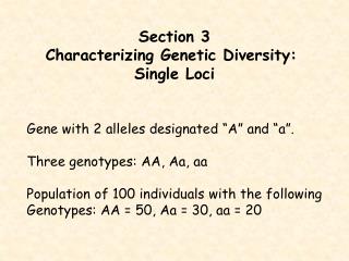
Section 3 Characterizing Genetic Diversity: Single Loci

Section 3 Characterizing Genetic Diversity: Single Loci Gene with 2 alleles designated “A” and “a”. Three genotypes: AA, Aa, aa Population of 100 individuals with the following Genotypes: AA = 50, Aa = 30, aa = 20

Genotypic frequencies -- General formula: f(AA) = NAA/N -- > 50/100 = 0.5 f(Aa) = NAa/N -- > 30/100 = 0.3 f(aa) = Naa/N -- > 20/100 = 0.2

Allele Frequencies: AA = 50, Aa = 30, aa = 20 Note, every individual carries two copies of the gene thus, the total number of alleles is 2N. p = frequency of “A” and q = frequency of “a”. The frequency of “A” is: p = (50 + 50 + 30)/200 = 0.65

Frequency of “a” is: q = (20 + 20 + 30)/200 = 0.35 Note: p + q = 1 therefore, an equivalent formula is: p = f(AA) + 0.5f(Aa) and q = 0.5f(Aa) + f(aa)

Hardy-Weinberg Equilibrium: under certain conditions, allele and genotypic frequencies will remain constant in a population from one generation to the next. Assumptions of Hardy-Weinberg Equilibrium: Organism in question is diploid Reproduction is sexual Generations are non-overlapping Panmixia Population size is infinitely large, or at least large enough to avoid stochastic errors

Migration (immigration/emigration) is negligible No mutation Natural selection does NOT affect the gene under consideration Hardy-Weinberg equilibrium is simple but provides the basis for detecting deviations from random mating, testing for selection, modeling the effects of inbreeding and selection, and estimating allele frequencies.

Single autosomal locus in a diploid organism with discrete generations. Initially consider a locus with only two alleles “A” and “a” with initial frequencies “p” and “q”. Designate frequencies of genotypes AA, Aa, and aa as P, H, and Q, respectively. Random Union of Gametes: Many marine invertebrates release their gametes into the sea and the gametes find one another and combine at random.

Sperm a q A p Allele Frequency Aa pq AA p2 A p E G G aa q2 Aa pq a q Note: p2 + 2pq + q2 = (p + q)2 = 1

Testing for deviations from H.W.E H.W.E serves as a null hypothesis and tells us what to expect if nothing interesting is happening. If we sample a population and find that the predictions of H.W.E are not met, then we can conclude that one or more of the assumptions is violated.

Chi-square test of “Goodness of Fit” 2 = (observed - expected)2/expected Example: You are studying a population of African elephants and assay the entire population (N = 260) for the ADH locus and find that the population contains only two alleles (F and f) with the following genotypic counts: FF = 65, Ff = 125, ff = 70

Step 1: Determine allele frequencies: p = F = (65 + 65 + 125)/520 = 0.4904 q = f = 1 - p = 1 - 0.4904 = 0.5096 Step 2: Calculate Expected genotypic freq.: P = p2 = (0.4904)2 = 0.2405 H = 2pq = 2(0.4904)(0.5096) = 0.4998 Q = q2 = (0.5096)2 = 0.2597

Step 3: Calculate chi-square statistic: O E (O-E)2/E P 65 0.2405 X 260 = 62.53 0.098 H 125 0.4998 X 260 = 129.95 0.189 Q 70 0.2597 X 260 = 67.52 0.091 2 = 0.378 Step 4: Compare calculated 2 with tabled 2: Degrees of freedom 3(# of genotypes) - 1(constant) - 1(#parameters) = 1

Look up critical values for 2 statistic: Level of Significance D.f. 0.05 0.01 0.001 1 3.84 6.64 10.83 2 5.99 9.21 13.82 3 7.82 11.34 16.27 Calculated 2 (0.378) is less than tabled value therefore we fail to reject the null hypothesis.

Cautionary notes about testing for deviations from H.W.E: Caution 1: If we find a population does not deviate from Hardy-Weinberg Equilibrium, we cannot conclude that no evolutionary forces are operating. Caution 2: The ability of the chi-square test to detect significant deviations from Hardy-Weinberg equilibriums is very weak.

Caution 3: Deviations from Hardy-Weinberg expectations gives us not information about the kinds or directions of the evolutionary forces operating.

Deviations from H.W.E There are two types of non-random mating, those Where mate choice is based on ancestry (inbreeding and crossbreeding) and those whose Choice is based upon genotypes at a particular Locus (assortative and disassortative mating).

Inbreeding: Is of major importance in conservation genetics as it leads to reduced reproductive fitness. When related individuals mate at a rate greater then expected by random mating, the frequency of heterozygotes is reduced relative to H.W.E. Avoidance of inbreeding and cross-breeding can lead to higher than expected heterozygosities.

Assortative and Disassortative Mating: the preferential mating of like-with-like genotype is called “assortative” mating. The mating of unlike genotypes is referred to as “disassortative” mating. In general, assortative mating leads to increased homozygosity, while disassortative mating increases heterozygosity, relative to H.W. expectations.

Fragmented populations: Allele frequencies diverge in isolated populations due to chance and selection. This results in an overall deficiency of heterozygotes, even when individual populations are themselves in H.W.E

Linkage Disequilibrium: In large, randomly mating populations at equilibrium, alleles at different loci are expected to be randomly associated. Consider loci A and B with alleles A1, A2, and B1, B2, and frequencies pA, qA, pB, qB, respectively. These loci and alleles form gametes A1B1, A1B2, A2B1, and A2B2. Under random mating and independent assortment, These gametes will have frequencies that are the Product of their allele frequencies, A1B2 = pAqB.

Random association of alleles at different loci is referred to as “Linkage Equilibrium”. Non-random association of alleles among loci is referred to as “Linkage Disequilibrium”. Chance events in small populations, population bottlenecks, recent mixing of different populations, and selection all may cause non-random associations among loci.

Loci that show deviations from linkage equilibrium in large randomly mating populations are often subject to strong forces of natural selection. In small populations, neutral alleles that have no selective differences between genotypes may behave as if they are under selection due to non-random association with alleles at nearby loci that are being strongly selected.

Linkage disequilibrium is of importance in populations of conservation concern as: Linkage disequilibrium will be common in threatened species as their population sizes are small. Population bottlenecks frequently cause linkage disequilibrium. Evolutionary processes are altered when there is linkage disequilibrium.

Functionally important gene clusters exhibiting linkage disequilibrium (such as MHC) are of major importance to the persistence of threatened species. Linkage disequilibrium is one of the signals that can be used to detect admixture of differentiated populations. Linkage disequilibrium can be used to estimate genetically effective population sizes.

Consider an example where two different monomorphic populations with genotypes A1A1B1B1 and A2A2B2B2 are combined and allowed to mate at random. Each autosomal locus is expected to attain individual H.W.E. in one generation. However, alleles at different loci do not attain linkage equilibrium frequencies in one generation, they only approach is asymptotically at a rate dependent on the recombination frequency between the two loci.

In this example of the pooled population, assume: 70% of pooled population isA1A1B1B1 30% of pooled population is A2A2B2B2 equal number of females & males of both genotypes. Only two gametic types are produced: A1B1, A2B2 Next generation: A1A1B1B1, A1A2B1B2, A2A2B2B2 These loci are clearly in linkage disequilibrium.

In subsequent generations, two other possible gametic types A1B2 and A2B1 are generated by recombination in the multiply heterozygous genotype. For example, A1B1//A2B2 heterozygotes produce recombinant gametes A1B2 and A2B1 at frequencies of 1/2c, where c is the rate of recombination and non-recombinant A1B1, A2B2 gametes in frequencies 0.5(1-c). Eventually, all 9 possible genotypes will be formed and attained at equilibrium frequencies.

Until equilibrium is reached, genotypes will deviate from their expected frequencies. Linkage disequilibrium is the deviation of gametic frequencies from their equilibrium frequencies. The measure of linkage disequilibrium D is the difference between the product of the frequencies of the A1B1and A2B2 gametes (referred to as r and u) and the product of the frequencies of the A1B2 and A2B1gametes (s and t): D = ru - st

Actual freq. r s t u 1.0 Equil. freq. pAqA pAqB qApB qAqB 1.0 Disequilibrium: D = ru - st Numerical Example: pA = 0.70, qA = 0.30, pB = 0.70, qB = 0.30 Actual freq. 0.70 0.00 0.00 0.30 Equil. freq. 0.7X0.7 0.7X0.3 0.3X0.7 0.3X0.3 0.49 0.21 0.21 0.09 Disequilibrium D = (0.7 X 0.3) - (0.0 X 0.0) = 0.21

Dmax = 0.25 and occurs when: r = 0.5, s = 0.0, t = 0.0, u = 0.5 Dmin = -0.25 and occurs when: r = 0.0, s = 0.5, t = 0.5, u = 0.0 Under equilibrium, ru = st and D = 0.

Many different measures of disequilibrium. Lewontin (1964) suggested D’, which is: D’ = D / Dmax Where, Dmax is the maximum D possible for a given set of allele frequencies at the two loci.

Dmax is equal either to the lesser of A1B2 (=s) or A2B1 (=t) if D is positive or to the lesser of A1B1 (=r) or A2B2 (=u) if D is negative. The advantage of this measure is that it ranges from -1.0 to 1.0, regardless of the allele frequencies at the two loci.

Gamete Freq. Allele Freq. A1B1 A1B2 A2B1 A2B2 D D’ 0.5 0.0 0.0 0.5 0.25 1.0 0.4 0.1 0.1 0.4 0.15 0.6* A1=B1=0.5 0.25 0.25 0.25 0.25 0.0 0.0 0.1 0.4 0.4 0.1 -0.15 -0.6 0.0 0.5 0.5 0.0 -0.25 -1.0 0.9 0.0 0.0 0.1 0.09 1.0 A1=B1=0.9 0.85 0.05 0.05 0.05 0.04 0.44 0.81 0.09 0.09 0.01 0.0 0.0 0.0 0.9 0.1 0.0 -0.09 -1.0 A1=B2=0.9 0.05 0.85 0.05 0.05 -0.04 -0.44* 0.09 0.81 0.01 0.09 0.0 0.0 A1=0.1,B1=0.5 0.1 0.0 0.4 0.5 0.05 1.0 0.05 0.05 0.45 0.45 0.0 0.0

Example 1:A1=B1=0.5 A1B1 A1B2 A2B1 A2B2 Actual Gametic Freq: 0.4 0.1 0.1 0.4 Equilib. Gametic Freq: 0.25 0.25 0.25 0.25 D = (A1B1 X A2B2) - (A1B2 X A2B1) D = (0.4 X 0.4) - (0.1 X 0.1) = 0.16 - 0.01 = 0.15 D’ = D/Dmax = 0.15/0.25 = 0.6

Example 2:A1=B2=0.9 A1B1 A1B2 A2B1 A2B2 Actual Gametic Freq: 0.05 0.85 0.05 0.05 Equilib. Gametic Freq: 0.09 0.81 0.01 0.09 D = (A1B1 X A2B2) - (A1B2 X A2B1) D = (0.05 X 0.05) - (0.85 X 0.05) = 0.0025 - 0.0425 = -0.04 D’ = D/Dmax = -0.04/0.09 = -0.44

Linkage disequilibrium decays as recombination produces underrepresented gametes. The rate of decay depends upon recombination frequency as follows: Dt = D0(1 - c)t Linkage disequilibrium declines rapidly for unlinked loci, with approximate linkage equilibrium reached in five generations. Conversely, decay of disequilibrium is slow for closely linked loci.

When linkage disequilibrium has been observed in a population, it has often been attributed to some type of multilocus selection. This assumption may not be valid because a number of other factors can affect linkage disequilibrium including: recombination genetic drift mutation gene flow inbreeding

Expected heterozygosity (He) = Gene diversity: For a single locus with two alleles, He = 2pq When more than two alleles, it is simpler to Calculate He as: k He = 1 - pi2 i=1 Where k = number of alleles

If sample sizes are smaller than 50 individuals: k He = 2N(1 - pi2)/(2N - 1) i=1 Where N is the number of individuals sampled. Gene diversity (He) is usually reported in Preference to observed heterozygosity as it is Less affected by sampling.

Conservation biologists are often concerned with changes in levels of genetic diversity over time, as loss of genetic diversity is one indication that the population is undergoing inbreeding and losing its evolutionary potential. Heterozygosity is often expresses as the proportion of heterozygosity retained over time. Ht/H0 where Ht is level of heterozygosity at generation t and H0 is the level at some time earlier, referred to as time 0.

For example, H0 may be the heterozygosity before a population crash and Ht after the crash. Then 1 - (Ht/H0) reflects the proportion of heterozygosity lost as a result of the crash.

Section 3 Characterizing Genetic Diversity: Single Loci