1d dynamics
V(x). 1d dynamics. 1 steady state:. 3 steady states:. 1d dynamics: saddle-node and cusp bifurcations. Similar systems:. Langmuir, enzyme. cut along m 2 =const. Exothermic reaction. General 2-variable system. Dynamical system Stationary solution Jacobi matrix Stability conditions.

1d dynamics
E N D
Presentation Transcript
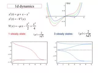
V(x) 1d dynamics 1 steady state: 3 steady states:
1d dynamics: saddle-node and cusp bifurcations Similar systems: Langmuir, enzyme cut along m2=const Exothermic reaction
General 2-variable system • Dynamical system • Stationary solution • Jacobi matrix • Stability conditions
Modified Volterra – Lotka system Modified prey–predator system accounting for saturation effects Stationary states Determinant of Jacobi matrix existence: k < 1 Trace of Jacobi matrix stability: c > 1 – 2k instability possible if k < 0.5 Hopf bifurcation: c = 1 – 2k {0, 0}, {1, 0}, {k, (1 - k) (c + k)} – k, –1 + k, (1 – k) k 1 – k, – k,
k=0.3, c=0.5 k=0.3, c=0.7 Hopf bifurcation at c=0.4 k=0.3, c=0.3 k=0.3, c=0.39
Dynamics near Hopf bifurcation Compute: Jacobi matrix at the bifurcation pointc = 1 – 2k eigenvalues eigenvectors U, U* Periodic orbit Slow dynamics: a = u(t), <<1 = m+ iw du /dt = u( –|u|2) Polar representation: u=(r/)eiq dr/dt = r(m– r2) dq/dt = w
Generalized Hopf bifurcation dr/dt = r(m1 + m2 r2 – r4) dq/dt = w1+ w2 r2 Complex rep:u=r eiq du/dt = u(1 + 2 |u|2 – |u|4) k = mk + iwk snp subcritical dr/dt = r(m– r2) dq/dt = w Complex rep: du/dt = u( – |u|2) = m+ iw Generic Hopf bifurcation supercritical Hopf
Bifurcation diagrams pitchfork supercritical Hopf generalized Hopf subrcritical Hopf
Global bifurcations Saddle-loop (homoclinic) Saddle-Node Infinite PERiod (Andronov)
Dynamics with separated time scales excitable oscillatory bistable biexcitable