Logical Foundations of Artificial Intelligence
550 likes | 730 Vues
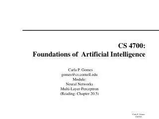
Logical Foundations of Artificial Intelligence. Markov Logic II. Markov Logic II. Summary of last class Applications Weight learning Formula learning. Markov Networks. Smoking. Cancer. Undirected graphical models. Asthma. Cough. Log-linear model:. Weight of Feature i. Feature i.

Logical Foundations of Artificial Intelligence
E N D
Presentation Transcript
Logical Foundations of Artificial Intelligence Markov Logic II
Markov Logic II • Summary of last class • Applications • Weight learning • Formula learning
Markov Networks Smoking Cancer • Undirected graphical models Asthma Cough • Log-linear model: Weight of Feature i Feature i
Inference in Markov Networks • Goal: Compute marginals & conditionals of • Exact inference is #P-complete • Conditioning on Markov blanket of a proposition x is easy, because you only have to consider cliques (formulas) that involve x : • Gibbs sampling exploits this
MCMC: Gibbs Sampling state← random truth assignment fori← 1 tonum-samples do for each variable x sample x according to P(x|neighbors(x)) state←state with new value of x P(F) ← fraction of states in which F is true
Capture the Flag Basics Logistic regression Hypertext classification Information retrieval Entity resolution Hidden Markov models Information extraction Statistical parsing Semantic processing Bayesian networks Relational models Robot mapping Planning and MDPs Practical tips Applications
Constraints • Player location critical for recognizing events • Capture requires players to be within an arm's reach • Consumer grade GPS loggers do not appear to have required accuracy • Error: 1 – 10 meters, typically 3 meters • Relative error: no better! • Differences in individual units much larger than systematic component of GPS error
Difficult Example • Did player 7 capture player 12 or player 13? • Can we solve this problem ourselves?
Difficult Example • 40 seconds later, we see: • 13 isn't moving • Another defender, 6 isn't trying to capture 13 • 12 is moving • Therefore, 7 must have captured 13!
Approach • Solve localization and joint activity recognition simultaneously for all players • Inputs: • Raw GPS data from each player • Spatial constraints • Rules of Capture the Flag • Output: • Most likely joint trajectory of all players • Joint (and individual) activities
Relational Reasoning • This is a problem in relational inference • Estimate of each player's location & activities affects estimates for other players • Rules of the game are declarative and logical • A player might cheat, but the rules are the rules! • Tool: Markov Logic (Domingos 2006) • Statistical-relational KR system • Syntax: first-order logic + weights • Defines a conditional random field
Comparison • Baseline • Snap to nearest 3 meter cell • If A next to B on A's territory, A captures B • Expect high recall, low precision • Baseline+States • Like baseline, but keep memory of players state {captured, not captured} • Expect better precision, possibly lower recall • 2-Stage Markov Logic Model • Find most likely explanation using ML theory about location • Use as input to ML theory about capture • Unified Markov Logic Model • Find most likely explanation using entire axiom set
Capture The Flag Dataset • 3 games • 2 teams, 7 players each • GPS data logged each second • Games are 4, 14, and 17 minutes long
Results for Recognizing Captures Sadilek & Kautz AAAI 2010
Uniform Distribn.: Empty MLN Example: Unbiased coin flips Type:flip = { 1, … , 20 } Predicate:Heads(flip)
Binomial Distribn.: Unit Clause Example: Biased coin flips Type:flip = { 1, … , 20 } Predicate:Heads(flip) Formula:Heads(f) Weight: Log odds of heads: By default, MLN includes unit clauses for all predicates (captures marginal distributions, etc.)
Multinomial Distribution Example: Throwing die Types:throw = { 1, … , 20 } face = { 1, … , 6 } Predicate:Outcome(throw,face) Formulas:Outcome(t,f) ^ f != f’ => !Outcome(t,f’). Exist f Outcome(t,f). Too cumbersome!
Multinomial Distrib.: ! Notation Example: Throwing die Types:throw = { 1, … , 20 } face = { 1, … , 6 } Predicate:Outcome(throw,face!) Formulas: Semantics: Arguments without “!” determine arguments with “!”. Also makes inference more efficient (triggers blocking).
Multinomial Distrib.: + Notation Example: Throwing biased die Types:throw = { 1, … , 20 } face = { 1, … , 6 } Predicate:Outcome(throw,face!) Formulas: Outcome(t,+f) Semantics: Learn weight for each grounding of args with “+”.
Logistic Regression Logistic regression: Type: obj = { 1, ... , n } Query predicate: C(obj) Evidence predicates:Fi(obj) Formulas:a C(x) biFi(x) ^ C(x) Resulting distribution: Therefore: Alternative form:Fi(x) => C(x)
Text Classification page = { 1, … , n } word = { … } topic = { … } Topic(page,topic!) HasWord(page,word) !Topic(p,t) HasWord(p,+w) => Topic(p,+t)
Text Classification Topic(page,topic!) HasWord(page,word) HasWord(p,+w) => Topic(p,+t)
Hypertext Classification Topic(page,topic!) HasWord(page,word) Links(page,page) HasWord(p,+w) => Topic(p,+t) Topic(p,t) ^ Links(p,p') => Topic(p',t) Cf. S. Chakrabarti, B. Dom & P. Indyk, “Hypertext Classification Using Hyperlinks,” in Proc. SIGMOD-1998.
Information Retrieval InQuery(word) HasWord(page,word) Relevant(page) InQuery(w+) ^ HasWord(p,+w) => Relevant(p) Relevant(p) ^ Links(p,p’) => Relevant(p’) Cf. L. Page, S. Brin, R. Motwani & T. Winograd, “The PageRank Citation Ranking: Bringing Order to the Web,” Tech. Rept., Stanford University, 1998.
Entity Resolution Problem: Given database, find duplicate records HasToken(token,field,record) SameField(field,record,record) SameRecord(record,record) HasToken(+t,+f,r) ^ HasToken(+t,+f,r’) => SameField(f,r,r’) SameField(f,r,r’) => SameRecord(r,r’) SameRecord(r,r’) ^ SameRecord(r’,r”) => SameRecord(r,r”) Cf. A. McCallum & B. Wellner, “Conditional Models of Identity Uncertainty with Application to Noun Coreference,” in Adv. NIPS 17, 2005.
Entity Resolution Can also resolve fields: HasToken(token,field,record) SameField(field,record,record) SameRecord(record,record) HasToken(+t,+f,r) ^ HasToken(+t,+f,r’) => SameField(f,r,r’) SameField(f,r,r’) <=> SameRecord(r,r’) SameRecord(r,r’) ^ SameRecord(r’,r”) => SameRecord(r,r”) SameField(f,r,r’) ^ SameField(f,r’,r”) => SameField(f,r,r”) More: P.Singla & P. Domingos, “Entity Resolution with Markov Logic”, in Proc. ICDM-2006.
Hidden Markov Models obs = { Obs1, … , ObsN } state = { St1, … , StM } time = { 0, … , T } State(state!,time) Obs(obs!,time) State(+s,0) State(+s,t) => State(+s',t+1) Obs(+o,t) => State(+s,t)
Information Extraction • Problem: Extract database from text orsemi-structured sources • Example: Extract database of publications from citation list(s) (the “CiteSeer problem”) • Two steps: • Segmentation:Use HMM to assign tokens to fields • Entity resolution:Use logistic regression and transitivity
Information Extraction Token(token, position, citation) InField(position, field, citation) SameField(field, citation, citation) SameCit(citation, citation) Token(+t,i,c) => InField(i,+f,c) InField(i,+f,c) <=> InField(i+1,+f,c) f != f’ => (!InField(i,+f,c) v !InField(i,+f’,c)) Token(+t,i,c) ^ InField(i,+f,c) ^ Token(+t,i’,c’) ^ InField(i’,+f,c’) => SameField(+f,c,c’) SameField(+f,c,c’) <=> SameCit(c,c’) SameField(f,c,c’) ^ SameField(f,c’,c”) => SameField(f,c,c”) SameCit(c,c’) ^ SameCit(c’,c”) => SameCit(c,c”)
Information Extraction Token(token, position, citation) InField(position, field, citation) SameField(field, citation, citation) SameCit(citation, citation) Token(+t,i,c) => InField(i,+f,c) InField(i,+f,c) ^ !Token(“.”,i,c) <=> InField(i+1,+f,c) f != f’ => (!InField(i,+f,c) v !InField(i,+f’,c)) Token(+t,i,c) ^ InField(i,+f,c) ^ Token(+t,i’,c’) ^ InField(i’,+f,c’) => SameField(+f,c,c’) SameField(+f,c,c’) <=> SameCit(c,c’) SameField(f,c,c’) ^ SameField(f,c’,c”) => SameField(f,c,c”) SameCit(c,c’) ^ SameCit(c’,c”) => SameCit(c,c”) More: H. Poon & P. Domingos, “Joint Inference in Information Extraction”, in Proc. AAAI-2007. (Tomorrow at 4:20.)
S VP NP NP V N Det N John ate the pizza Statistical Parsing • Input: Sentence • Output: Most probable parse • PCFG: Production ruleswith probabilities E.g.: 0.7 NP → N 0.3 NP → Det N • WCFG: Production ruleswith weights (equivalent) • Chomsky normal form: A → B C or A → a
Statistical Parsing • Evidence predicate:Token(token,position) E.g.: Token(“pizza”, 3) • Query predicates:Constituent(position,position) E.g.: NP(2,4) • For each rule of the form A → B C:Clause of the form B(i,j) ^ C(j,k) => A(i,k) E.g.:NP(i,j) ^ VP(j,k) => S(i,k) • For each rule of the form A → a:Clause of the form Token(a,i) => A(i,i+1) E.g.:Token(“pizza”, i) => N(i,i+1) • For each nonterminal:Hard formula stating that exactly one production holds • MAP inference yields most probable parse
Semantic Processing • Weighted definite clause grammars:Straightforward extension • Combine with entity resolution:NP(i,j) => Entity(+e,i,j) • Word sense disambiguation:Use logistic regression • Semantic role labeling:Use rules involving phrase predicates • Building meaning representation:Via weighted DCG with lambda calculus(cf. Zettlemoyer & Collins, UAI-2005) • Another option:Rules of the form Token(a,i) => Meaningand MeaningB ^ MeaningC ^ … => MeaningA • Facilitates injecting world knowledge into parsing
Semantic Processing Example: John ate pizza. Grammar: S → NP VP VP → V NP V → ate NP → John NP → pizza Token(“John”,0) => Participant(John,E,0,1) Token(“ate”,1) => Event(Eating,E,1,2) Token(“pizza”,2) => Participant(pizza,E,2,3) Event(Eating,e,i,j) ^ Participant(p,e,j,k) ^ VP(i,k) ^ V(i,j) ^ NP(j,k) => Eaten(p,e) Event(Eating,e,j,k) ^ Participant(p,e,i,j) ^ S(i,k) ^ NP(i,j) ^ VP(j,k) => Eater(p,e) Event(t,e,i,k) => Isa(e,t) Result:Isa(E,Eating), Eater(John,E), Eaten(pizza,E)
Bayesian Networks • Use all binary predicates with same first argument (the object x). • One predicate for each variable A: A(x,v!) • One clause for each line in the CPT andvalue of the variable • Context-specific independence:One Horn clause for each path in the decision tree • Logistic regression: As before • Noisy OR: Deterministic OR + Pairwise clauses
Robot Mapping • Input:Laser range finder segments (xi, yi, xf, yf) • Outputs: • Segment labels (Wall, Door, Other) • Assignment of wall segments to walls • Position of walls (xi, yi, xf, yf)
MLNs for Hybrid Domains • Allow numeric properties of objects as nodes E.g.: Length(x), Distance(x,y) • Allow numeric terms as features E.g.: –(Length(x)–5.0)2 (Gaussian distr. w/ mean = 5.0 and variance = 1/(2w)) • Allow α=β as shorthand for –(α–β)2 E.g.: Length(x) = 5.0 • Etc.
Robot Mapping SegmentType(s,+t) => Length(s) = Length(+t) SegmentType(s,+t) => Depth(s) = Depth(+t) Neighbors(s,s’) ^ Aligned(s,s’) => (SegType(s,+t) <=> SegType(s’,+t)) !PreviousAligned(s) ^ PartOf(s,l) => StartLine(s,l) StartLine(s,l) => Xi(s) = Xi(l) ^ Yi(s) = Yi(l) PartOf(s,l) => = Etc. Cf. B. Limketkai, L. Liao & D. Fox, “Relational Object Maps for Mobile Robots”, in Proc. IJCAI-2005. Yf(s)-Yi(s)Yi(s)-Yi(l) Xf(s)-Xi(s) Xi(s)-Xi(l)
Practical Tips • Add all unit clauses (the default) • Implications vs. conjunctions • Open/closed world assumptions • How to handle uncertain data:R(x,y) => R’(x,y)(the “HMM trick”) • Controlling complexity • Low clause arities • Low numbers of constants • Short inference chains • Use the simplest MLN that works • Cycle: Add/delete formulas, learn and test
Learning Markov Networks • Learning parameters (weights) • Generatively • Discriminatively • Learning structure (features) • In this tutorial: Assume complete data(If not: EM versions of algorithms)
No. of times feature i is true in data Expected no. times feature i is true according to model Generative Weight Learning • Maximize likelihood or posterior probability • Numerical optimization (gradient or 2nd order) • No local maxima • Requires inference at each step (slow!)
Pseudo-Likelihood • Likelihood of each variable given its neighbors in the data • Does not require inference at each step • Consistent estimator • Widely used in vision, spatial statistics, etc. • But PL parameters may not work well forlong inference chains
Discriminative Weight Learning • Maximize conditional likelihood of query (y) given evidence (x) • Approximate expected counts by counts in MAP state of y given x No. of true groundings of clause i in data Expected no. true groundings according to model