Download
1 / 26
270 likes | 392 Vues
Simulation of cars waiting at a toll booth using Scilab. Jianfeng Li Institute of Industr ial Process Control, Control Science and Engineering Department,zhejiang university 2006.9. Introduction The queue system’s performance index The optimal number of servers Simulation Conclusion.

E N D
Simulation of cars waiting at a toll booth using Scilab Jianfeng Li Institute of Industrial Process Control, Control Science and Engineering Department,zhejiang university 2006.9
Introduction • The queue system’s performance index • The optimal number of servers • Simulation • Conclusion
Introduction Queuing theory • It is the study of the waiting line phenomena. • It is a branch of applied mathematics utilizing concepts from the field of stochastic processes. • It is the formal analysis of this phenomenon in search of finding the optimum solution to this problem so that everybody gets service without waiting for a long time in line.
Introduction • The queue system is composed of the arrival process the queue discipline the service process • If there is one server in all service process, it is called single-server system. • If the server number is more than one and each sever can serve customers independently, it is called multi-server system
Introduction • Usually, the service system is evaluated by performance indexes, such as • Service intensity • Average queuing length • Average queuing time • Average stay time • Probability of the service desks being idle • The probability of the customers having to wait
Introduction • The basic service process is the following: busy the customers arrive queuing system waiting line free served according to the prescribed queuing discipline finished leave the system
Introduction • The terms customer, server, service time, and waiting time may acquire different meanings in different applications. • In this article • The customers are cars arriving at a toll booth • The servers are the workers in the tool booth • The service times are the payment times
The queue system’s performance index • In the simulation of cars waiting at a toll booth, some necessary condition assumptions and notation definitions should be made. • Assumptions: • The arrival time and service time follow exponential distribution. • The waiting queue is infinite.
The queue system’s performance index • Notations: • λ: the arrival rate of the car • μ: the service rate of the car • ρ: the service intensity • Ls: the average quantity of cars in the system • Lq: the average quantity of cars in the waiting queue • Ws: the average time of each car stay in the system • Wq: the average time of each car stay in the waiting queue
The queue system’s performance index according to John DC Little’s formula, we only discuss two usual models. • Standard M/M/1 service model. • Standard M/M/C service model.
Standard M/M/1 service model • The arrival time and service time of cars can be discretional distribution. • The number of server is one. • The car source and service space are infinite. • The queuing discipline is first come first service.
Standard M/M/1 service model • So the major performance indexes are: • Service intensity: • Probability of the server being idle: • Probability of n cars in the system:
Standard M/M/C service model • The arrival time and service time of cars can be discretional distribution. • the number of server is C and they are parallel connection . • Servers work independently and the average service rate is the same. • The car source and service space are infinite. • The queuing discipline is first come first service.
Standard M/M/C service model • So the major performance indexes are: • Service intensity: • Probability of the server being idle: • The average quantity of cars in the waiting queue: • The average quantity of cars in the system: • The average time of each car stay in the system: • Probability of the car has to waiting after arriving:
The optimal number of servers • Step 1, according to , find out the initialization number of servers ; • Step 2, compute the performance indexes, such as the average quantity of cars in the waiting queue, the average time of each car stay in the system, and the average time of each car stay in the waiting queue. Comparing them with desired indexes, if it is dissatisfied, go to step 3; otherwise, the optimal number of servers is N and the process is end. • Step 3, let , go to step 2.
Simulation • In this system, the arrival time and service time of car are similar to the exponential distribution. • Assume that the left time of the ith car is the begin service time of the (i+1)th car. • All the events can be classified to two sorts: one is the arrival event of cars; the other is the leave event of car. • When the arrival event and the leave event occur at a same time, disposed the former first.
Simulation • In Scilab simulation environment, the average arrival rate of cars, the average service rate of cars and the simulation terminate time are given by the following:
Simulation • In the simulation platform we present, the draw mode of SCILAB is set to be animate all along so that a gliding process can be observed.
Simulation • The animation demo can be described as:
Simulation • Assume that the terminate time of simulation is 240 sec. • The average arrival rate is 0.18. • And the average service rate is 0.1. • The minimum servers’ number can be found out: =1. • The queuing discipline is first come first serve.
Simulation The simulation results can be calculated: • The average quantity of cars in the waiting queue is: 15 • The max quantity of cars in the waiting queue is: 26 • The average quantity of cars in the system is: 16 • The average time of each car stay in the waiting queue is: 146sec • The average time of each car stay in the system is: 162sec • All the served cars number is: 22
Simulation • Let , the number of server become 2. • The simulation process is similar to the above single servers systems. The different is that, in the simulation, when the second car arrival, it can be serviced immediately because there are two servers in the system. So the car will pass the toll booth with less waiting time.
Simulation The simulation results with two servers are: • The average quantity of cars in the waiting queue is:3 • The max quantity of cars in the waiting queue is: 6 • The average quantity of cars in the system is: 4 • The average time of each car stay in the waiting queue is: 29sec • The average time of each car stay in the system is: 41sec • All the served cars number is: 42
Simulation • Comparing the above results with desired performance index, it is found that when there are two servers, the demands can be satisfied. • So, it is recommended to open two servers.
Conclusion • Queuing theory have been used in almost every domain of social and natural science as a tool to solve many problems. In this article, queuing theory is used to solve the problem of cars waiting in a tool booth. • Using the tools of Scilab, the simulation of a single queuing multi-servers system is done and the optimal number of server is obtained.
The end Thank you!