Stand Structure - Definitions
Western Mensurationists 2013 Leavenworth, WA, USA Where’s Waldo? Stand structure indices and maximum density relationships. Ian Moss , PhD, RPF Tesera Systems Inc. Valerie LeMay, PhD, RPF University of British Columbia.

Stand Structure - Definitions
E N D
Presentation Transcript
Western Mensurationists 2013 Leavenworth, WA, USAWhere’s Waldo? Stand structure indices and maximum density relationships.Ian Moss, PhD, RPF Tesera Systems Inc.Valerie LeMay, PhD, RPF University of British Columbia
“It may be that Reineke’s index is not a good measure of density, but it is still the best we have. At least it does not lead to confusion between overstocked and understocked stands of the same species. However the relationship between the number of trees and diameter may not be as simple as Reineke believed.” Boris Zeide 2005
Stand Structure - Definitions = tree dbh – Dg (relative dbh; not dbh/Dg) = proportion of basal area per hectare relative dbh (cumulative distribution) = proportion of trees per hectare relative dbh (cumulative distribution)
Objectives • To evaluate relationships between Stand Structure Indices (SSI) and Reineke’s (1933) SDI, i.e. Stand Structure = f (N, Dg, SSI ) where SSI = f(pG, pN | rDbh) ? • … and Maximum Density ~ f(Dg, SSI)?
Stand Structure Indices • Three Indices: • Gini Coefficient (e.g. Bonan 1988; GINI) • Lorenz Area and Lorenz Maximum (LA or LM analogous to GINI) • Cumulative Distribution Index (CDI)
GINI For a given plot, i, the average absolute difference in size (x = dbh) amongst all pairs of individual trees, j & m, scaled in proportion to the mean (xbar= mean tree dbh). Bonan, G. B. 1988. The size structure of theoretical plant populations: spatial patterns and neighborhood effects. Ecology 69:1721-1730. Sen, A. 1973. On economic inequality. Clarendon, Oxford. Cited in Weiner, L. 1985. Size hierarchies in experimental populations of annual plants. Ecology 66(3):743-752.
Lorenz Area Line of absolute equality _-_ Line of perfect uniformity rev. J. Maximally Bimodal -_- Duduman, G. 2011. A forest management planning tool to create highly diverse uneven-aged stands. Forestry 84(3):301-314.
CDI Numerical integration at standard rDbh intervals (1 cm) Trees ranked (large to small)
Method of Evaluation: Part I • Plot level distributions: pGandpN vs. rDbh • Fuzzy C-Means classification: 5, 10, and 20 classes. • Find best index to explain differences amongst classes. • Also classify plot-level Lorenz Curve’s (pGat fixedpNintervals); compare results. • Classes ranked and renumbered according to LA (low to high).
The Data 1/10thhectare plots 174 Combined variable and fixed radius plots 247 Fdi leading species 233 Pl leading species 184 Other (SX, VV) 4
Results: Indices Interpretations Coefficient of Variation Bendel, R.B., Higgins, S.S., Teberg, J.E., and Pyke, D.A. 1989. Comparison of skewness coefficient, coefficient of variation, and GINI coefficient as inequality measures within populations. Oecologia 78:394-400.
Method of Evaluation: Part II • Use Frontier regression (frontier in R) sfa routine to evaluate maximum density as a function of Dg, structural index (SSI), and Dg*SSI with, and without species differentiation. Coelli, T. and Henningsen, A. 2012. Stochastic Frontier Analysis. R package ‘frontier’. Version 0.997-14. http://frontier.r-forge.r-project.org/ [accessed May 27 2013] .
Conclusion I • The Cumulative Distribution Index (CDI) • Fits within the concept of SDI (N, Dg) as residual information describing the degree of difference amongst diameter distributions. • Is a reliable index of differences in stand structure. • Provides better differentiation of plots with respect to leading species (vs. LA and GINI). • Probably includes better accounting for differences related to the shapes of distributions (i.e., skewness) that is not included in LA, and may come at a cost of being less precise with respect to CV.
Conclusion II • Maximum Density: • Differences related to species can/may be explained by structural differences. • Differences in species (can) explain differences in maximum density ; differences in stand structure may (Pl) or may not (Fd) have a demonstrable significant effect. • The maximum density differences are most pronounced with respect to changes in stand structure in the region of low CDI, i.e. stands with trees distributed within a narrow range of diameters.
Question When compared with PL, FD has higher maximum density due to: … greater complexity in stand conditions? … more shade tolerance? … a combination of the above? … nature of dataset?


