Download

1 / 63
640 likes | 940 Vues
Topology Management Ad hoc and Sensor Networks. The Need for Topology Management. What is it? The physical or logical interconnection pattern of a network Topology schemes in wired networks: Bus Star Ring Why do we need different schemes in sensor networks?

E N D
Topology Management Ad hoc and Sensor Networks
The Need for Topology Management • What is it? • The physical or logical interconnection pattern of a network • Topology schemes in wired networks: • Bus • Star • Ring • Why do we need different schemes in sensor networks? • location of sensors is not deterministic • resource constraints
The Need for Topology Management • Energy/Power consumption • Interference • Throughput • Connectivity
Mobility-Adaptive Protocols for Managing Large Ad hoc Networks [Basagni+ 2001] Motivation for Backbone Architecture • essential for management of large ad hoc networks • helps generate the minimum possible overhead for construction and maintenance of the backbone network • can provide efficient solution for mobility and node/link failures in very large ad hoc networks
B-Protocol Also known as backbone protocols Sets up and maintains a connected network (B-network) B-network convey the time-sensitive network management information from every node in the network with minor overhead and in a timely manner Comprises two major tasks: (a) B-nodes selection (b) B-links establishment Nodes that are not selected as B-nodes are termed F- nodes that belong to the flat network Mobility-Adaptive Protocols for Managing Large Ad hoc Networks Proposed B-Protocol Description
Executed at each node based on a node’s own weight Weight is computed based on what is most critical to that node for the specific network application The highest weight of a node is more suitable to be a B-node A node knows Its own identifier (ID) and weight Ids, weights and roles (B-node or F-node) of one-hop neighbors Once a node b determines its role as B-node, all its neighbors may become the F-nodes served under bunless they have decided to join another node B-nodes selection is adaptive to node mobility and changes in its local status Mobility-Adaptive Protocols for Managing Large Ad hoc Networks B-nodes Selection
6(1) 2(3) 4(9) 1(6) 7(5) 3(2) 5(8) 8(1) Mobility-Adaptive Protocols for Managing Large Ad hoc Networks B-nodes Selection Illustrative Example: Numbers represent node IDs and numbers within parentheses represent the node weights
Mobility-Adaptive Protocols for Managing Large Ad hoc Networks B-nodes Selection Illustrative Example: 6(1) 2(3) 4(9) B-node B-node 1(6) 7(5) 3(2) 5(8) 8(1) B-node
Determines the inter-B-nodes links to be established in order for the network to be connected Two types of B-links: Physical – when a direct link between B-nodes at most three hops away can be established without involving intermediate F-nodes (via power control or directional antenna) Virtual – when a direct link between B-nodes at most three hops away cannot be established. In this case, virtual link is implemented among two B-nodes by a corresponding physical path with at most three links The rules stated follow the theorem proven in [Chlamtac ’96] Mobility-Adaptive Protocols for Managing Large Ad hoc Networks B-links Establishment
Mobility-Adaptive Protocols for Managing Large Ad hoc Networks B-links Establishment Theorem 1 [Chlamtac ’96]: Given a set B of network nodes such that no two of them are neighbors and every other node has a link to a node in B, then a connected backbone is guaranteed to arise if each node in B establishes links to all other nodes in B that are at most three hops away. Moreover, these links are all needed for the deterministic guarantee in the worst case, in the sense that if any of them is left out then it is not true anymore that the arising backbone is connected for any underlying flat network.
Each node in flat network knows only its one-hop neighbors. This induces the minimum possible overhead B-link establishment is run at each B-node only with no knowledge of the surrounding B-nodes. Again, this induces the minimum overhead Every B-node serves a number of F-nodes each of which is at most three-hops away. B-node selection protocol guarantees that all the F-nodes are served by only one neighboring B-node There are no two B-nodes that are neighbors in the flat network. This guarantees that B-nodes are evenly distributed in the network B-node selection is based on the node’s current status (weight) Mobility-Adaptive Protocols for Managing Large Ad hoc Networks Properties of B-protocol
The B-network is always connected provided that the underlying flat network is connected B-protocols takes into account different technologies and mechanisms that can be used to link the B-nodes in the network. Two types of B-links are provided; namely physical and virtual links. Physical links are used when there is a direct link between B-nodes at most three hops away and virtual links are used when there is a direct link cannot be established Mobility-Adaptive Protocols for Managing Large Ad hoc Networks Properties of B-protocol
A simulator used for an ad hoc network of nodes ranges 100 - 1000 Nodes can freely move around in a rectangular region (a grid) Node movements are discretized to grid units of 1 meter A node determines its direction randomly by choosing between its current direction (with 75% probability) and uniformly among all other directions (with 25% probability) When a node hits a grid boundary, it bounces back into the region with an angle determined by the incoming direction Fixed transmission range of each node (250 m) and the grid size have been chosen to obtain a good network connectivity Each packet contains the time-stamped, node identified weight of the sending node. All packets are sent for the one-hop neighbors only Mobility-Adaptive Protocols for Managing Large Ad hoc Networks Simulation Environment
kis the total number of F-nodes a B-node can serve at any point in time Three cases: k < n (where n is total number of nodes in network) k < 4 k < 8 Mobility-Adaptive Protocols for Managing Large Ad hoc Networks Simulation Results Figure 1: Number of B-nodes (% w.r.t the number of the network nodes)
kis the total number of F-nodes a B-node can serve at any point in time Three cases: k < n (where n is total number of nodes in network) k < 4 k < 8 Mobility-Adaptive Protocols for Managing Large Ad hoc Networks Simulation Results Figure 2: Number of B-links (%) when a physical link between any two B-nodes can be established directly.
kis the total number of F-nodes a B-node can serve at any point in time Three cases: k < n (where n is total number of nodes in network) k < 4 k < 8 Mobility-Adaptive Protocols for Managing Large Ad hoc Networks Simulation Results Figure 3: Number of B-links (%) when a link between B-nodes is implemented by a physical path with at most three hops away
Optimizing Sensor Networks in the Energy-Latency-Density Design Space[Schurgers+ 2002] • Describes • a topology management technique that is power efficient • energy, Latency and Density trade-offs • Provides • a theoretical analysis of these techniques, including a mathematical formulation that can be used to design a network with required energy, latency and density configuration • a hybrid solution with existing topology management scheme (GAF) to provide energy saving of over two order of magnitude • The proposed new topology management scheme is called • STEM (Sparse Topology and Energy Management)
Optimizing Sensor Networks in the Energy-Latency-Density Design Space[Schurgers+ 2002] • Two states for sensor nodes: • Monitoring State • Transfer State • Most of the time a sensor remains in monitoring state (i.e. sensing environment) • When an event occurs, nodes come into transfer mode and transfer their data
Optimizing Sensor Networks in the Energy-Latency-Density Design Space[Schurgers+ 2002] • Issues: • Nodes must listen periodically for call to duty (i.e transfer) • But if they poll periodically on the same frequency, it will collide with other data transfer • Solution: • Use two radios, one for polling while the other for data transfer • STEM-B (Beacon Approach): • Initiator sends a stream of beacon packets to poll a target with initiator and target MAC addresses • Target node sends acknowledgement on receiving the packet • Target node turns its transfer radio on
Optimizing Sensor Networks in the Energy-Latency-Density Design Space[Schurgers+ 2002] • STEM-T (Tone Approach) • Initiator sends a wake up tone • Every node receiving that tone starts its data transfer radio • No need to send acknowledgement • Every node in the neighborhood of initiator wakes up • STEM/GAF Hybrid • GAF proposes a scheme in which a sensor network is divided in a grid • One node in a region has its radio on, others have it turned off • Nodes alternate the responsibility of being the active node • GAF uses network density to conserve energy • Assuming the active node to be the virtual node, STEM can be used on the virtual node to manage whole network
Optimizing Sensor Networks in the Energy-Latency-Density Design Space[Schurgers+ 2002] Advantages: • Highly efficient in environments where events are rare • Flexible in term of design trade-off for energy, latency and density • Transition from monitoring state to transfer state is easily achieved • No synchronization required • Can be use with other topology management schemes like GAF Disadvantages: • Continuous polling consumes energy • Not suitable for highly reactive environments • Requires extra radio on sensor nodes • Suggestions/Improvements/Future Work: • Analysis of STEM with clustered networks
ASCENT: Adaptive Self-Configuring sEnsor Networks Topologies [Cerpa+ 2002] • In ASCENT, the nodes coordinate to exploit the redundancy provided by high density to extend the overall system lifetime • Nodes achieve self-configuration to establish a topology that provides communication and sensing coverage under energy constraints • Each node examines its connectivity and adapts its participation in the multi-hop network topology based on the operating region • The node • Signals when it detects high message loss, requesting additional nodes to join the network to continue relaying messages • Reduces its duty cycle if high messages losses are detected due to collisions • Probes local communication environment and only joins to the multi-hop routing infrastructure if it is useful
ASCENT: Adaptive Self-Configuring sEnsor Networks Topologies [Cerpa+ 2002] • Sensor nodes do local processing to reduce communication and energy costs • Challenges arises from the increased level of dynamics(systems and environmental) • One of the most important challenge arises from energy constraints imposed by unattended systems • These systems must be long-lived and operate without manual intervention • They need to self-configure and adapt to environmental dynamics and some terrain conditions may result regions with non-uniform communication density • These issues can be addressed by deploying redundant nodes and designing algorithms to use redundancy to extend the system lifetime • Scaling challenges are associated with spatial coverage and robustness • Central vs. Distributed • When energy is constraint and environment is dynamic, distributed approaches are preferable and practical
ASCENT: Adaptive Self-Configuring sEnsor Networks Topologies [Cerpa+ 2002] • Scalable wireless sensor networks require to avoid large amounts of data being transmitted over long distances • ASCENT applies well-known techniques from MAC layer protocols to the problem of distributed topology formation • Imagine a habitat monitoring sensor network that is deployed in remote forest • The deployed systems must confer with the following conditions • Ad-hoc deployment • Energy constraints • Unattended operation under dynamics • If we use too few nodes initially: • the distance between neighboring nodes will be too far • packet loss rate may increase • energy required to transmit over larger distances may be prohibitive
ASCENT: Adaptive Self-Configuring sEnsor Networks Topologies [Cerpa+ 2002] • If we use all deployed nodes simultaneously: • system will expand unnecessary energy • nodes interfere with each other by congesting the channel • ASCENT does not use localized distributed algorithm to find a single solution • Adaptive self-configuration using localized is suited to problem spaces which have a vast number of possible solutions (in this case, large solution spaces means dense node deployment) • ASCENT has the following two assumptions: • Carrier Sense Multiple Access (CSMA) MAC protocol • Possibilities for resource contention when too many neighboring nodes participate in the multi-hop network • Reacts when links have high packet loss • Does not detect or repair network partitions and assumes that there is enough node density to connect the entire region
ASCENT: Adaptive Self-Configuring sEnsor Networks Topologies [Cerpa+ 2002] • Two essential contributions of ASCENT design are: • Adaptive techniques that allow applications to configure the topology based on the needs while saving energy to extend network lifetime. The techniques do not assume a specific model or fairness, degree of connectivity, or capacity required • Self-configuring techniques that react to operating conditions are measured locally. It does not assume any specific radio propagation model, geographical distribution of nodes, or routing mechanisms used • ASCENT Design • Adaptively elects active nodes from all the nodes • Active nodes stay awake always and participate in routing while the other nodes remain passive and periodically checks if they should become active
Help Messages Data Message Passive Neighbor Active Neighbor Source Sink ASCENT: Adaptive Self-Configuring sEnsor Networks Topologies [Cerpa+ 2002] • ASCENT Design • Initially, only some nodes are active while other are passively listening to packets but not transmitting • When source starts transmitting data packets towards the sink, the sink gets high message loss from the source due to limited radio range, called communication hole • The receiver gets high packet loss due to poor connectivity with the sender Figure 2(a): Communication Hole
ASCENT: Adaptive Self-Configuring sEnsor Networks Topologies [Cerpa+ 2002] • ASCENT Design • Sink start sending help messages to neighbors that are in listen-only mode, called passive neighbors, to join the network • When a neighbor receive a help message, it decides to join the network or not • If the node joins, it becomes an active neighbor and signals the existence of a new active neighbor to other passive neighbors by sending a neighbor announcement message • It continues until the number of active nodes stabilizes on a certain value and the cycle stops
Neighbor Announcements Messages Data Message Sink Source Sink Source ASCENT: Adaptive Self-Configuring sEnsor Networks Topologies [Cerpa+ 2002] • ASCENT Design • When the process is completed, the newly joined nodes participate in the data delivery process from source to sink more reliably • The process will be repeated in the case of network event (e.g., node failure) or environmental effect (e.g., new obstacle) causes message loss Figure 2(b-c): Self-configuration transition and final state
Test Active after Tt neighbors > NT (high ID for ties); or loss > loss T0 • neighbors < NT and • loss > LT • loss < LT & help Sleep after Tp Passive after Ts ASCENT: Adaptive Self-Configuring sEnsor Networks Topologies [Cerpa+ 2002] ASCENT State Transactions NT: neighbor threshold LT: loss threshold T?: state timer values (p: passive, s: sleep, t: test) DL: Data loss rate
ASCENT: Adaptive Self-Configuring sEnsor Networks Topologies [Cerpa+ 2002] • ASCENT State Transactions • Initially, a random timer turns on the nodes to avoid synchronization • Node initializes to test state: • Sends data and routing control messages • Sets up a timer, Tt and sends neighbor announcement messages • Moves into passive state if the conditions are met before Tt expires • When Tt expires, it enters to active state • The reasoning behind the test state is to probe the network to decide whether the addition of a new node would improve connectivity • On entering the passive state, node: • Sets up a timer Tp and when Tp expires, it enters to sleep state • If before Tp expires, it enters to test state only if the conditions are met • Nodes in passive state can hear all packets transmitted, but no routing or data packets are forwarded in this state since this is listen-only state
ASCENT: Adaptive Self-Configuring sEnsor Networks Topologies [Cerpa+ 2002] • ASCENT State Transactions • The reasoning behind the passive state is to gather information about the state of the network without causing interference with other nodes • Nodes in passive and test states update the number of active neighbors and data loss rates • In passive states, the nodes still consume energy since the radio is on • The nodes in sleep state turns the radio off, sets up timer Ts and goes to sleep • When Ts expires, the nodes moves into passive state • A node in the active state continuous to forward data and routing packets until it runs out of energy
ASCENT: Adaptive Self-Configuring sEnsor Networks Topologies [Cerpa+ 2002] • ASCENT Parameters Tuning • ASCENT has many parameters and the choices are left to the applications such as a particular application may trade energy savings for greater sensing coverage • Neighbor Threshold (NT): • Determines the average connectivity if the network • Tradeoff between energy consumed and/or level of interference (packet loss) vs. desired sensing coverage • Loss Threshold (LT): • Determines the maximum amount of data loss an application can tolerate before requesting help to improve network connectivity • This value is highly application dependent
ASCENT: Adaptive Self-Configuring sEnsor Networks Topologies [Cerpa+ 2002] • ASCENT Parameters Tuning • Test timer (Tt), Passive timer (Tp), Sleep timer (Ts): • Determines the maximum time a node remains in test, passive, sleep states • Tradeoff between power consumption vs. decision quality
SPAN: An Energy-Efficient Coordination Algorithm for Topology Maintenance in Ad hoc Wireless Networks [Chen+ 2002] • SPAN is a power saving technique for multi-hop ad hoc networks that reduces energy consumption with the consideration of maintaining the capacity or connectivity of the network • It is distributed and randomized algorithm in which the nodes make local decisions on whether to sleep or join to the backbone • Each node decides based on an estimate of how many neighbors will benefit from it being awake and the energy available to it • Improvement in the system lifetime increases along with the ratio of idle-to-sleep energy consumptions • Non-coordinators remain in power saving mode and periodically check to see if they should wake up and become coordinators
SPAN • A good power saving technique for ad hoc networks should have the following: • Allow as many as nodes to turn their radios off most of the time • Forward packets between any source and destination with the minimum possible delay than if all nodes were awake • Distributed algorithm where having each node making local decisions • Backbone formed by the awake nodes should provide close to total capacity as the original networks such that congestion can be avoided • Do not make many assumptions about the link layer’s facilities for sleeping and work with any link layer that provides sleeping and periodic polling • Inter-operate correctly with any routing algorithm being used • SPAN fulfills all the above requirements • Each node makes periodic local decisions to sleep or stay awake as a coordinator and participate in the forwarding backbone topology
SPAN • In order to keep the same level of capacity of the original network, a node may volunteer to become a coordinator if it figures out from the local information gathering that two of its neighbors cannot communicate directly or through one or two existing coordinators • In order to keep the number of coordinators low and rotate this role amongst all nodes, each node delays sending message about its desire to become a coordinator by a random time interval • The decision is based on two factors: • the remaining battery energy • the number of pairs of neighbors it can connect together • This allows SPAN to maintain capacity-preserving backbone at any time with the nodes consuming about the same level of energy • SPAN also scales well with the number of nodes
SPAN • SPAN Design • The goals of SPAN includes: • Ensures enough coordinators to be elected such that each node is in radio range of at least one coordinator • Rotates coordinators to ensure that all nodes provides equal support to achieve global connectivity • Increases the network lifetime, preserves the capacity with minimum latency by minimizing the number of elected coordinators • Coordinators are elected based on local available information • SPAN is proactive such that each node periodically broadcasts HELLO messages which contains the node’s status (coordinator or not), its current coordinators, and its current neighbors • From these HELLO messages, each node keeps tracks of a list of the node’s neighbors and coordinators, and for each neighbor, a list of its neighbors and coordinators
SPAN • Coordinator Announcement • Each non-coordinator node periodically determines whether it should become a coordinator or not • The coordinator eligibility rules ensures that the network is covered with sufficient number of coordinators • Coordinator Eligibility Rule • A non-coordinator node should become a coordinator if it figures out from the local • information gathering that two of its neighbors cannot communicate directly or through • one or two existing coordinators • If many nodes are willing to become coordinators, SPAN solves this contention by delaying coordinator announcement with a randomized backoff delay • Each node selects a delay value and delays sending HELLO message indicating the desire to become coordinator for that amount of time • At the end of the delay, the node reevaluates its eligibility based on the HELLO messages received from neighbors and if it is still eligible, it makes announcement
SPAN • Coordinator Announcement • At the end of the delay, the node reevaluates its eligibility based on the HELLO messages received from neighbors and if it is still eligible, it makes announcement • Consider a case where all the nodes have the same level of energy which means that only topology is considered in the decision of becoming a coordinator • Consider a case where the nodes have unequal energy left Er = energy remaining at node Ni = number of neighbors for node i Em = maximum amount of energy T = round-trip delay for packet Ci = number of new connections through node i R = random number in [0, 1] Eq. 1 Eq. 2
SPAN • Coordinator Announcement • In Eq. 1, if nodes with high Ci become coordinators, total number of coordinators needed would be less to ensure that every node in the network is covered • Therefore, the nodes with a high Ci values should volunteer for coordinator position quicker than those with smaller Ci • In Eq. 2, the node with large value of (Er/Em) is expected to volunteer quicker to become a coordinator than the nodes with smaller ratio in order to assure the fairness
SPAN • Coordinator Withdrawal • Each node periodically checks whether it should withdraw as a coordinator • A node withdraws if all of its neighbors can reach each other directly or with one or more coordinators • For fairness, after some period of time, a coordinator withdraws and declares itself as a tentative coordinator if all neighbors can reach each other via other neighbors, even if these are not coordinators (allows neighbors to act as coordinators) • A tentative coordinator is still used to forward packets and described coordinator announcement algorithm treats tentative coordinators as non-coordinator nodes • A coordinator nodes gives its neighbors the opportunity to become coordinators by declaring itself as tentative coordinator • A coordinator maintains its position as tentative for WT time, where WT is the maximum value of Eq. 2 which is • WT = 3 x Ni x T
SPAN • Coordinator Withdrawal • If the coordinator has not withdrawn within WT time period, it clears its tentative bit • In order to prevent node to drain its battery completely, the amount time a node acts as a coordinator before turning on its tentative bit is proportional to the amount of energy it has, indicated as (Er/Em)
SPAN Simulation Results
Distributed Topology Control in Wireless Sensor Networks with Asymmetric Links [Liu+ 2003] • Topology Control • Does not describe a new topology • Provides a mechanism to build certain topology • Distributed • No central control or central source of information • Asymmetric Links • Due to the presence of heterogeneous devices
Distributed Topology Control in Wireless Sensor Networks with Asymmetric Links [Liu+ 2003] • Objective • Reachability between any two nodes is guaranteed to be like initial topology • Nodal power consumption is minimized
Distributed Topology Control in Wireless Sensor Networks with Asymmetric Links [Liu+ 2003] • Model • Network of heterogeneous sensors (called nodes) • Nodes deployed in a two dimensional plane • Each node equipped with omni-directional antenna with adjustable transmission power • Nodes have different maximum power • Pi = Transmission Power of Node i • Pimax = Maximum Transmission Power of Node i • Pij = Transmission Power required for node i to reach j • Lij = Asymmetric link from i to j • G = (V, L) : directed graph of topology with max power • G is strongly connected
Distributed Topology Control in Wireless Sensor Networks with Asymmetric Links [Liu+ 2003] • Algorithm • Fully distributed with no synchronization required • Takes G as input and produces G’ where G’ has: • Same bi-directional reachability • Consumes minimum power • Phases • Establishing the vicinity topology • Deriving the minimum power vicinity tree • Propagation of transmission powers • Optimizations
Distributed Topology Control in Wireless Sensor Networks with Asymmetric Links [Liu+ 2003] • Establishing the vicinity topology • Node i broadcasts initialization request (IRQ) with Pimax • Vi is the set of nodes that receive the message {i.e. locationi, Pimax} • Each node j in Vi sends initialization reply (IRP) message {i.e. locationj, Pjmax} • If Pjmax > Pij , j can reach I with single hop Lji • Otherwise find a multi-hop path to reach i • Given the knowledge of location and max power of itself and all vicinity nodes, node i can determine the vicinity edges • Node i establishes a vicinity topology , Gi =(Vi, Ei)
Distributed Topology Control in Wireless Sensor Networks with Asymmetric Links [Liu+ 2003] • Deriving Minimum Power Vicinity Tree • Derive Minimum power path in Gi, to reach from a node i to node j using Dijkstra or Bellman-Ford algortihms based on sum of power consumption on that path. • Compute it for each node in Vi to obtain minimum-power vicinity tree, • Gis = (Vi, Eis)