
a 1 +/+
Appendix 1: Laurens W.J. Bosman, Johannes C. Lodder, Klaartje Heinen, Sabine Spijker, Arjen van Ooyen, Thomas W. Rosahl and Arjen B. Brussaard. a 1 +/+. a 1 -/-.

a 1 +/+
E N D
Presentation Transcript
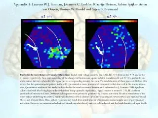
Appendix 1: Laurens W.J. Bosman, Johannes C. Lodder, Klaartje Heinen, Sabine Spijker, Arjen van Ooyen, Thomas W. Rosahl and Arjen B. Brussaard a1 +/+ a1 -/- Photodiode recordings of visual cortex slices loaded with voltage-sensitive dye (VSD, RH 414) from an a1 +/+ and an a1 -/- mouse respectively. Time lapse recording of the changes in fluorescence upon electrical stimulation (5 x at 40 Hz), applied to the white matter (arrow), whereafter the signal can be seen spreading towards the apex. The total duration of these movies is 160 ms. It is shown that the spatiotemporal pattern in the wild type animals is more pronounced compared to that observed in the mutant mouse slice. Quantitative analysis of this has been described in the result section of Bosman et al. submitted to J. Neurosci. VSD signals are color-coded with blue being hyperpolarized and red being optimally depolarized. Signal to noise is around 1-2 % DF. As shown previously (Contreras & Llinas, 2001) optical responses were primarily generated by synaptic activation Electrical stimulation of the white matter underlying the cortical mantle excites both cortical afferent (primarily consistingof corticocortical and thalamocortical fibers) and efferent fibers.Thus, optical responses may result from antidromic or orthodromic(monosynaptic and/or polysynaptic) activation. However, on occasionsuch electrical stimuli may also directly activate cells in layer6 and the basal dendrites of layer 5cells.
Appendix 2: Laurens W.J. Bosman, Johannes C. Lodder, Klaartje Heinen, Sabine Spijker, Arjen van Ooyen, Thomas W. Rosahl and Arjen B. Brussaard a1 +/+ a1 -/- Integrate-and-fire model (conform Van Ooyen et al. 1992) simulations of 6400 neocortex neurons (pyramidal versus interneurons 70:30%) being randomly connected in a circle surround fashion, with realistic AMPA versus GABAA receptor open time kinetics. On the left the a1 +/+ condition and on the right the a1 -/- condition was tested, by compared IPSC decay time constants of 8 versus 6 ms respectively. It is shown that the patches of active cells in the network at equilibrium on the left cell occur with larger area of spreading excitation compared to the right side, conform the VSD recording in Bosman et al. submitted to J.Neurosci.
Using a simple model of the visual cortex, we tested whether the smaller spread of network activity in a1 -/- mice could be a direct result of the longer decay time of the inhibitory postsynaptic current (IPSC) in these mice. The model described in Van Ooyen et al. (1992) is used to build a network with integrate-and-fire neurons and roughly the same connectivity pattern as in the cortex. We constructed two networks that are exactly the same (i.e., have exactly the same connectivity structure) except for their IPSC decay time constant. One network has an IPSC decay time constant of 8 ms (representing a1 -/- mice), and the other a decay time of 6 ms (representing a1 +/+ mice). Network Model. The network is composed of excitatory (e) and inhibitory (i) cells, which are randomly placed on a two-dimensional grid, the boundaries of which are connected to each other. Given the distribution of excitatory and inhibitory cells, each cell is connected to a number of target cells, which are randomly chosen with uniform probability within a circular field. The radius of this field depends on the type of outgoing connection. The e to e connections are short range, the e to i connections are long range, and the i to e and i to i connections are medium range. For each cell, the strength and number of outgoing connections also depend on the type of connection. Neuron Model.The membrane potential of a neuron at time t, V(t), is expressed relative to the resting potential Er and is calculated using where Se = Ge / Gr and Si = Gi / Grrepresent the strengths of the excitatory and inhibitory inputs, respectively, expressed as ratios of the synaptic conductances Ge and Gi to the resting conductance Gr ; and Me = Ee - Er and Mi = Ei – Er , where Ee and Ei are the excitatory and inhibitory driving potentials. The values of Se and Siare taken to decay according to the time courses of EPSC and IPSC: where De and Di are constants (0 < D < 1) and Ie(t) and Ii(t) are the momentary excitatory and inhibitory inputs at time t, with time partitioned into discrete intervals. Each time interval in the model corresponds to about 1 ms. The generation of an action potential is reduced to a threshold rule: if V(t) exceeds the firing threshold q, the cell fires. After firing, there is a refractory period, simulated by putting q up to Me and then letting it decrease back to the default value.
Parameters.The network is composed of 80 x 80 cells, 30% inhibitory (i) and 70% excitatory (e). For the e to e connections: number = 24, radius = 2, and strength = 0.06. (Note that a target cell can be innervated by multiple connections from the same neuron.) For the e to i connections: number = 20, radius = 15, and strength = 0.05. For the i to e connections: number = 74, radius = 5, and strength = 0.05. For the i to i connections: number = 6, radius = 5, and strength = 0.05. (Radius is expressed in number of cells; connection strength is expressed as ratio of the synaptic conductance to the resting conductance; see section Neuron Model.) Me= 73 mV, and Mi = 0 mV (shunting inhibition). The value of De is such that Se decays with a time constant t of 5 ms (EPSC decay time). In the network representing the a1 -/- mice, Si decays with a time constant of 8 ms (IPSC decay time); in the a1 +/+ network, it decays with a time constant of 6 ms. The connectivity structures of both networks are exactly the same. Results. The movies show the spread of network activity following an initial stimulation of the central cell for one time step; then stimulation is stopped. The strengths of the connections are such that the network remains active without external stimulation. Activity in the network spreads out until an equilibrium state is reached in which a patch of cells is active that does no longer expand (at that point we have stopped the movies). The size of this patch depends on the decay time of the IPSC. In the a1 -/- network (long IPSC decay time), the size of the patch of active cells at equilibrium is smaller than in the a1 +/+ network (shorter decay time), in accordance with what has been found experimentally. In the model, when an excitatory cell is stimulated, it recruits other cells in its neighborhood (the e to e connections are short range), so that activity expands. But at the same time, inhibitory cells farther away become activated (the e to i connections are long range), which in turn project back to excitatory cells (the i to e connections), inhibiting them. Thus, the active patch of cells becomes surrounded by a ring of inhibited excitatory cells (not visible as such in the movie because of shunting inhibition) and active inhibitory cells, which, if the ring is closed, prevents further expansion of activity. A longer IPSC decay time means that the i to e connections are effectively stronger, so that the excitatory cells become more inhibited and the expansion of activity is stopped earlier. Note that the IPSC decay time influences inhibitory input not only on excitatory cells but also on inhibitory cells (the i to i connections). A long IPSC decay time also means that the i to i connections are effectively stronger, so that the inhibitory cells become less active and the excitatory cells less inhibited. However, the overall result of these two opposing effects is that inhibition becomes stronger and the spread of activity is reduced. In conclusion, we have shown that the experimentally observed reduced spread of network activity in a1 -/- mice could be a direct result of the longer IPSC decay time in these mice. References. Van Ooyen, A., Van Pelt, J., Corner, M. A., and Lopes da Silva, F. H. (1992). The emergence of long-lasting transients of activity in simple neural networks. Biol. Cybern. 67: 269-277.