Sample Size and Power Calculations
Sample Size and Power Calculations. Andy Avins, MD, MPH Kaiser Permanente Division of Research University of California, San Francisco. Why do Power Calculations?. Underpowered studies have a high chance of missing a real and important result Risk of misinterpretation is still very high

Sample Size and Power Calculations
E N D
Presentation Transcript
Sample Size and Power Calculations Andy Avins, MD, MPH Kaiser Permanente Division of Research University of California, San Francisco
Why do Power Calculations? • Underpowered studies have a high chance of missing a real and important result • Risk of misinterpretation is still very high • Overpowered studies waste precious research resources and may delay getting the answer [BTW: “Sample Size Calculations” ≡ “(Statistical) Power Calculations”]
A Few Little Secrets • Why, yes, power calculations are basically crap • Nothing more than educated guesses • Playing games with power calculations has a long and glorious history • So why do them? • You got a better idea? • Review committees don’t give you a choice • Can be enlightening, even if imperfect
Power Calculations • Purpose • Try to rationally guess optimal number of participants to recruit (Goldilocks principle) • Understand sample size implications of alternative study designs
The Problem of Uncertainty • If everyone responded the same way to treatment, we’d only need to study two people (one intervention, one control) • Uncertainty creeps in when: • When we draw a sample from a population • When we allocate participants to different comparison groups (random or not)
Thought Experiment • We have 400 participants • Randomly allocate them to 2 groups • Test if Group 1 tx does better than Group 2 tx • Throw all participants back in the pool, re-allocate them, and repeat the experiment • Truth: Group 1 tx IS better than Group 2 tx • We know this
Thought Experiment • Clinical Trial Run #1: 1>2 [Correct] • Clinical Trial Run #2: 1>2 [Correct] • Clinical Trial Run #3: 1=2 [Incorrect] • Clinical Trial Run #4: 1>2 [Correct] • Clinical Trial Run #5: 1=2 [Incorrect] • Clinical Trial Run #6: 2>1 [Incorrect] • Clinical Trial Run #7: 1>2 [Correct] • Clinical Trial Run #8: 1>2 [Correct] • ………
Thought Experiment • Repeated the thought experiment an infinite number of times • Result: • 70% of runs show 1>2 (correct result) • 30% of runs show 1=2 or 1<2 (incorrect result)
Thought Experiment • POWER of doing this clinical trial with 400 participants is 70% • Any ONE run of this clinical trial (with 400 participants) has about a 70% chance of producing the correct result • Any ONE run of this clinical trial (with 400 participants) has about a 30% chance of producing the wrong result
Bottom Line • If you only have a 70% chance of showing what you want to show (and you only have $$ for 400 participants): • Should you bother doing the study??
Power Calculations • Sample size calculations are all about making educated guesses to help ensure that our study: A) Has a sufficiently high chance of finding an effect when one exists B) Is not “over-powered” and wasteful
Error Terminology • Two types of statistical errors: • “Type I Error” ≡ “Alpha Error” • Probability of finding a statistically significant effect when the truth is that there is no effect • “Type II Error” ≡ “Beta Error” • Probability of not finding a statistically significant effect when one really does exist • Goal is to minimize both types of errors
Error Terminology Truth of Association Reject Ho when we shouldn't (this is fixed at 5%) Type I Error (α) Correct Observed Association Type II Error (β) Correct Don't reject Ho when we should (not fixed; this is a function of sample size)
Hypothesis Testing • Power calculations are based on the principles of hypothesis testing • Research question ≠ hypothesis • Device for forcing you to be explicit about what you want to show
Hypothesis Testing: Mechanics 1) Define the “Null Hypothesis” (Ho) • Generally Ho = “no effect” or “no association” • Assume it’s true • Basically, a straw man (set it up so we can knock it down) • reductio ad absurdum in geometry Example: There is no difference in the risk of stroke between statin-treated participants and placebo-treated participants.
Hypothesis Testing: Mechanics • 2) Define the “Alternative Hypothesis” (HA) • Finding of some effect • Can be one-sided or two-sided • One-sided: better/greater/more or worse/less • Two-sided: different • Which to choose? • One-sided: biologically impossible for other possibility, don’t care about other possibility (careful!) • Easier to get “statistical significance” with one-sided HA • When in doubt, choose a two-sided HA • Example: Statin treatment results in a different risk of stroke compared to placebo treatment
Hypothesis Testing: Mechanics 3) Define a decision rule • Virtually always: reject the null hypothesis if p<.05 • This cutpoint (.05) = “alpha level”
Hypothesis Testing: Mechanics 4) Calculate the “p-value” • Assume that Ho is true • Do the study / gather the data • Calculate the probability that we’d see (by chance) something at least as extreme as what we observed IF Ho was true
Hypothesis Testing: Mechanics 5) Apply the decision rule: • If p < cutpoint (.05), REJECT Ho • i.e., we assert that there is an effect • If p> cutpoint (.05), DO NOT REJECT Ho • i.e., we do not assert that there is an effect • Note: this is different from asserting that there is no effect (you can never prove the null)
Terminology Review • Null and Alternative Hypotheses • One-sided and Two-Sided HA • Type I Error (α) • Type II Error (β) • Power: 1 - β • p – value • Effect Size
The Normal Curve Probability
Ingredients Needed to Calculate the Sample Size • Need to know / decide: • Effect Size: d • SD(d) • Standardized Effect Size: d / SD(d) • Cutpoint for our decision rule • Power we want for the study • What statistical test we’re going to use • We can use all this information to calculate our optimal sample size
Where the Pieces Come From: d • d is the “Effect Size” • d should be set as the “minimum clinically important difference” (MCID) • This is smallest difference between groups that you would care about • Sources • Colleagues (accepted in clinical community) • Literature (what others have done) • Smaller differences require larger sample sizes to detect (danger: don’t fool yourself)
Where the Pieces Come From: SD(d) • Standard deviation of d • Generally, based on prior research • Literature (often not stated); can derive • Contact other investigators • +/- pilot study
Where the Pieces Come From: Cutpoint • Easy: written in stone (Thanks, RA Fisher) • Alpha = 0.05 • Need to state if one-sided or two-sided
Where the Pieces Come From: Power • Higher is better • You decide • Rules of thumb: • 80% is minimum reviewers will accept • Rarely need to propose >90% • Greater power requires larger samples
Outcome Variable Dichotomous Continuous Chi-Square t-test Dichotomous Predictor Variable t-test Correlation Coefficient Continuous Where the Pieces Come From: Statistical Test • A function of data types you will analyze
Finally, Some Good News • Someone else has done these calculations for us • “Sample Size Tables” • DCR, Appendix 6A – 6E (pp. 84 – 91) • Entire books • Power Analysis Software • PASS, nQuery, Power & Precision, etc • Websites (Google search)
Real-Life Example (Steroids for Acute Herniated Lumbar Disc) • Ho: There is no difference in the change in the ODI scores between two treatment groups. • Alpha: 0.0471 (two-tailed) • Beta: 0.1 (Power=90%) • Clinically relevant difference in ODI change scores: 7.0 • Standard deviation of change in ODI scores: 15.1 • Randomization ratio: 1:1 • Statistical test on which calculations are based: Student’s t-test • Number of participants required to demonstrate statistical significance = 101 per group; Total number required (two arms) = 202 • Number of participants required after accounting for 20% withdrawals = 244 • Based on a projected accrual rate of 8-10 participants per month, we anticipate that we will require approximately 2.25 years to fully recruit to this trial.
Power Calculations for a Descriptive Study • Goal: estimate a single quantity • Power: determines the precision of the estimate (i.e., the width of the 95% CI) • Greater power = better precision = narrower CI