Advanced Approaches to Tracking and Control in Servo Systems
Explore advanced methods for tracking and control in servo systems with examples like inverted pendulum and magnetic suspension. Learn about optimizing control gains and handling errors effectively. Discover strategies for stabilizing closed-loop systems and achieving desired reference states.


Advanced Approaches to Tracking and Control in Servo Systems
E N D
Presentation Transcript
Lecture 37. More on Tracking Alternate approach to tracking (what we saw Tuesday night) The new ritual Second order servo-motor The inverted pendulum from today’s PS (The magnetic suspension problem revisited)
With the choice we can write There is an alternate way to attack the tracking problem What we’ve done so far is find some ur such that It’s worth noting that this is not a method that will work for all reference states but it’s really good when it does work Alternatively we can find some Arsuch that as
What about Ar? Clearly the class of constant reference states has Ar = 0 which is the case for the example he works Let’s see how to do this for simple cases Suppose we have a one degree of freedom cart and we want it to go back and forth
We can look at a more complicated case Suppose we have a pair of second order equations with the state If we are to look for harmonic reference states
What about the magnetic suspension problem? The desired state is and we can write
Back to the general problem xr which we can diagram as A – Ar e u b A
We want e to go to zero We know how to make e go to zero in the absence of tracking We simply check for controllability, and then find relevant gains for a full state feedback control u =- gTe We can extend this idea by choosing u to depend on e and xr
Combine all of this And we can draw a diagram of this
xr A – Ar - bgrT e A –bgT
It is not all clear how this works, and As it happens it does not always work: we cannot always get e = 0 We have to settle for: The closed loop system (no explicit appearance of xr) asymptotically stable Some components of e going to zero The closed loop system means the system without xr The following argument is not the be all and end all — sometimes we can do better, but let’s look at it anyway
We have to do the g part first That will make the closed loop error go to zero Then we can move on to the gr part We cannot always do everything, so let’s look at what we can do Suppose that we have found g
We can ask that the derivative of the error goes to zero, from which is stable, hence invertible and we can solve for e, and write If xr is as big as the space, with k components, then e has kcomponents There are k components of gr but that turns out not to mean that I can fix this We’ll see this best in terms of examples.
We can make some of the error vanish — the output, as defined by c We get the nicest result when the output has as many elements as the input In our case we want to look at single input-single output (SISO) systems Put in the matrix dimensions to help us understand The left hand side is a scalar — that part of e that we make disappear
rearrange this to set it up as an equation for gr we want this to work for any xr that is a member of the set defined by Ar
c is not a square matrix, so it doesn’t have an inverse; we have to invert the entire matrix multiplying gr: is a scalar for a SISO system, so its inverse is very simple
Let me review the new method beginning at the very beginning, with a general nonlinear tracking problem A general single input tracking problem can be written We seek a control u to make this work. We only know how to do this for a linear model so we need to linearize the problem Find an equilibrium solution such that and linearize around it (Typically ) We can find
The linear problem is and we want some reference state Let The linearized problem becomes
Find an Ar such that we can replace the derivative of xr and then substitute that into the equations of motion We make up this matrix Write and substitute into the differential system where now we want to make e go to zero, leaving x = xr
We find g as we have done before: Find Q and check controllability Find T and its inverse and A1 = TAT-1 Find g to place poles at desired locations The new wrinkle is finding gr, which is going to reduce the forced error to zero We suppose that we can at least find a constant error vector e If that is so, then we can write an expression for the error 0
Ideally we would be able to choose gr such that the entire error vector is zero This is not possible in general, but sometimes it is possible It is worthwhile to look at the vector error to check If you can find gr that makes e vanish, then you are done If not, you can probably find some c such that cTe does vanish. In other words, you can usually make a single output error vanish which is often all you really need to do.
rearrange solve for gr
At this point you have determined both gain matrices by one method or another It is time to verify the control you have designed The original problem The control Some algebra The simulation
Summary of the summary Convert the problem to a mathematical formulation in state space Linearize if necessary Find the two gains g and gr Substitute the control into the original problem and assess its performance
the servo Motor Tracking Suppose we want to make a servo motor track a sine wave We neglect inductive effects, supposing that which leaves us with a second order system that we have seen before The problem is linear, so we can skip the linearization stage and proceed to the usual equations We have a reference state
the servo We can copy the second order motion equations from Lecture 24 where or
the servo The reference state is sinusoidal, and we can develop Aras I did sat the beginning and of course we still have
the servo We make the standard expansion and arrive at the error equation recall A is in companion form and B is close enough, so I can skip that exercise and write
the servo The two characteristic polynomials are From which we can determine the gains to place the poles Let’s think a little bit about where to place these poles We’ll think some more at the end of the day, if we have time, for now
We’re working on stabilizing the error equation independent of xr. This is a closed loop problem with eigenvalues and eigenvectors The poles govern their behavior.
the servo The original problem is a second order linear problem. As such it can be underdamped, overdamped or critically damped. We know that a critically damped system does not overshoot so maybe that is what we want to do Critically damped systems have two identical (negative, real) eigenvalues Let’s place both our poles at -1/t.
the servo We will need the closed loop matrix later, so let’s write that out here Now we can move on to construct the other gain Here’s the error equation for that 0 All the pieces we need are on the next slide, and we can build this
the servo In this case we can actually eliminate the entire error as formulated
the servo What does all this mean in terms of actual performance? It should be clear that there must be starting transients we are unlikely to start the motor on exactly the correct note We need to go back and solve the original problem with the control we have designed This is a two dimensional linear problem that lends itself to solution using the state transition matrix. Remember that?
the servo is solved by where In this case the solution is given by
the servo We’ll need some numbers for illustrative purposes: K = 1 = G is not unreasonable There’s an interesting interplay between the frequency the servo is to follow and the time constant of the “ordinary” gain g. We could explore this in Mathematica
magnetic suspension From Kuo BC Automatic Control Systems yis positive down Numerical parameters for later
magnetic suspension Manipulate the equations combine these input
magnetic suspension We want to linearize around the equilibrium solution
magnetic suspension The linear equations We can make a matrix equation out of this
magnetic suspension new gains: radius = 10
magnetic suspension Suppose that we want to have the ball oscillate around its equilibrium position I don’t think I can do this using the nonlinear equations of motion We can do this in the linearized formulation. I want y = x1 to oscillate: y = dsin(wt) I don’t actually care about the other elements of the state but I certainly have to make the velocity the derivative of the position the current is not so clear, but it will have to be harmonic I have a linear problem, if some of it is harmonic, then the whole thing must be harmonic
magnetic suspension We know a lot about the linearized system already: we know the eigenvalues and we know it’s controllable We even know that we can make it track by assigning a ur. So, let’s do it again using the new method