Download
1 / 17
170 likes | 235 Vues
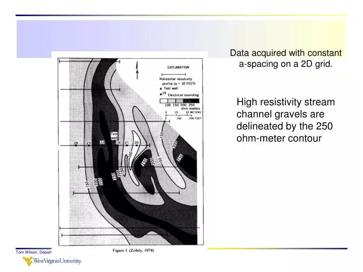
Data acquired with constant a-spacing on a 2D grid. High resistivity stream channel gravels are delineated by the 250 ohm-meter contour. Melted areas in permafrost Constant a-spacing. Profiling. Depth.

E N D
Data acquired with constant a-spacing on a 2D grid. High resistivity stream channel gravels are delineated by the 250 ohm-meter contour Tom Wilson, Department of Geology and Geography
Melted areas in permafrost Constant a-spacing Tom Wilson, Department of Geology and Geography
Profiling Depth Exploration depth remains constant and the measured variations in ground conductivity provide a view of relative variations in conductivity at the exploration depth Constant Spread Traverse Tom Wilson, Department of Geology and Geography
Location of gravel deposits in a clay alluvium Constant a-spacing Tom Wilson, Department of Geology and Geography
Tri-potential resistivity method 2a Can you compute the geometrical factors for these various electrode configurations? 3a -6a Tom Wilson, Department of Geology and Geography
Questions about the technique? Increase in apparent resistivity measured by the CCPP electrode array is actually an indicator of a low resistivity – perhaps water filled - fracture zone. Tom Wilson, Department of Geology and Geography
Case History Resistivity Profiling Surveys on the Hopemont Farm in Terra Alta, WV Survey performed by Eb Werner for Dr. Rauch Tom Wilson, Department of Geology and Geography
Survey was conducted for the City of Terra Alta to locate a water well. From Werner and Rauch Tom Wilson, Department of Geology and Geography
The tri-potential resistivity response over an air-filled fracture zone. Model data CPCP CPPC CCPP From Werner and Rauch Tom Wilson, Department of Geology and Geography
The Terra Alta surveys conducted by Werner and Rauch employed measurements at three different a-spacings - 10ft, 20 ft and 40 ft. • Lines were positioned to cross a photolineament and were from 250 to 500 feet in length. • Readings were made at 10 foot intervals. Things to avoid- Conductive materials buried or in contact with the ground. Buried telephone cables and metallic pipelines, fences, metallic posts and overhead power lines Tom Wilson, Department of Geology and Geography
Interpretation approach The apparent resistivity measurements made by Werner and Rauch were interpreted within the context of the tri-potential response predicted by the Carpenter model (see earlier figure). “.. The present problem involves only the confirmation of the existence and exact location of a fracture zone mapped from other information. ” “ … it is only necessary to locate anomalies characteristic of vertical discontinuities …” “ … the graphic plots were inspected visually for those anomaly responses ..” Anomalous areas were plotted on location maps. “Alignments of such anomalies at or near the location of the postulated fracture zone were accepted as confirmation of the existence of the fracture zone. Tom Wilson, Department of Geology and Geography
Sounding Coil spacing Midpoint Expanding Spread 40m 20m 10m 3.7m EM34 EM34 EM34 EM31 Surface 5.5m depth Exploration 15m depth Depth 30m depth 60mdepth Tom Wilson, Department of Geology and Geography
Northernmost site - site 1 (see earlier location map) Line 1 is highlighted in red below From Werner and Rauch Tom Wilson, Department of Geology and Geography
High resistivity would normally indicate what kind of fracture zone. N S The anomaly around 100 feet is considered to be “data noise” The feature at 320 feet is interpreted to be the “fracture zone” response. Note that this feature is not marked by highs in the CPPC and CPCP measurements Line 1 The 20 foot a-spacing profile reveals a more pronounced fracture zone anomaly at about 320 feet along the profile. The response suggests high reistivity Tom Wilson, Department of Geology and Geography From Werner and Rauch
Red dots locate prominent “fracture zone” anomalies observed on all three a-spacings Line 1 The blue line indicates the probable location of a major fracture zone. Given the 10 foot station spacing location of the zone is accurate to no more than ±5 feet Line 6 From Werner and Rauch Tom Wilson, Department of Geology and Geography
N S The fracture zone anomaly appears consistently on Line 6 at approximately 125 feet along the profile Line 6 The anomaly broadens as the a-spacing increases because electrodes in the array extend over the anomalous region at greater and greater distances from the array center point. From Werner and Rauch Tom Wilson, Department of Geology and Geography
Northernmost site - site 1 (see earlier location map) Line 1 is highlighted in red below From Werner and Rauch Tom Wilson, Department of Geology and Geography