Understanding Property Rights and Market Efficiency: Insights from Environmental Economics
This document explores the concept of property rights, detailing how they impact ownership, benefits, and costs associated with goods. It emphasizes the importance of well-functioning institutions for market efficiency and the allocation of property rights, particularly concerning environmental resources. The discussion includes case studies, such as sugar farming's effects on the Everglades, and examines externalities and the implications of property rights ownership for efficient market outcomes. The need for clear title and enforcement in property rights is underscored, especially in contexts like Latin America.

Understanding Property Rights and Market Efficiency: Insights from Environmental Economics
E N D
Presentation Transcript
Property Rights • A PROPERTY RIGHT is a title to, or ownership of, a good or bad. It entitles the owner to: • 1. Enjoy the benefits and costs of the good, and prevent others from doing so without compensation. • 2. Sell the good in a market and therefore transfer ownership and benefits and costs. Property rights, and thus the welfare theorems, require well-functioning institutions. Without a police force and functioning justice system, most goods are non excludable and are therefore under-provided in a market economy. • In many Latin American countries, it is difficult to obtain clear title to your property and keep squatters from using other’s land. Not surprisingly, such properties tend to be underdeveloped. • No one wants to risk building on the property when the property may be taken at any time. • No one talks about over-harvesting of cattle (clear property rights) the way they talk about over fishing.
A Who Should Be Assigned Property Rights? • In order for markets to function, the government must assign property rights when they are unclear, and then enforce the property rights. • For most goods, like land and housing, it is clear who to assign the property rights to. Environmental goods are less clear. • 1. Who should have rights to the stream, the farmer for irrigation or the fishing industry? • 2. Who should have rights to the land which contains an endangered species, the developer or the public?
1- Efficient Allocation • Let us compute the efficient allocation, and then see if assigning property rights to one party or another results in an efficient allocation. One recent example is sugar farming and the Everglades. • Suppose: • A farm produces sugar (S) and fertilizer run-off from the farm eventually ends up in the Everglades where it kills fish. A fishing company produces fishing trips (T) in the Everglades. • The cost of producing sugar is CS (S). • The cost of a fishing trip is CT (T, S): more sugar production makes fish more difficult to find, requiring more time on the boat, gas, etc. • We have an externality: farm production affects fishing without compensation. But there is an easy way to resolve this externality: merge the firms. The merged firm maximizes profits:
π = psS + pT T − CS (S) − CT (S, T) • Sugar production then increases until the price equals the marginal cost, but the marginal cost includes the higher cost of fishing production: • The merged firm produces the socially efficient amount of sugar (S∗), taking into account the marginal cost of production including the fishing costs.
2- Fishing company owns the property right • Suppose now the fishing company can charge the farmer for fertilizer runoff. Suppose the fishing company charges P′ for each unit of sugar produced per unit of the fertilizer which should always be made in terms of the quantity of the good or bad causing the externality. • Now how much runoff will the fishing company “supply”? The fishing company allows the sugar farmer to supply and additional unit of sugar if the revenues gained (P′) exceed the loss of profits that results from the sugar production. Otherwise it would be better to deny the farmer access and produce fish at a lower cost. Let MD be the “marginal damage "or the increase in costs to fishing caused by a small increase in sugar production. • Then the supply curve is: • Supply = dCT (S, T)/dT = MD(S)
Continue.. • Now how much sugar production will the farmer “demand” to produce? Recall the farmer gets Ps in revenue per unit of sugar and already faces MC (S) in costs per unit. Now she will produce if the marginal profits exceed the cost of producing. Hence the sugar farmer’s demand curve is: Demand = Ps −MC (S) = Ps − dCs (S)/dS Graphically, market for run off:
Continue.. • If payment is P′ = 0, the firm produces S0, but has an incentive to reduce production if the fishing company charges for runoff. • At SH > S∗, the sugar farmer has negative marginal profits. For unit SH, he receives Ps revenue less MC (SH) costs. But this is less than the P′ the sugar farmer must pay the fishing company. Thus the sugar farmer reduces production. • At SL < S∗ , the fishing company could make more profits by allowing runoff. The runoff cost the firm only MD(SL) in lost fishing profits, but that is more than made up for by the P′ in payments from the sugar farm. • Returning to the math, at the equilibrium, supply equals demand so: • Demand = Ps −MC (S) = Supply = MD orPs −MC (S) = MD(S) or • Ps = MC (S) +MD(S) we see that the efficient level of sugar is produced when the fishing company has the property right.
Continue. • Finally, looking at the above graph, we must have: P′= MD(S) = dCT (S,T)/dT
3 Farmer Owns the Property Right • Now let us suppose that the farmer owns the right to dump into the Everglades. The fishing company can always pay the farmer not to produce, however. Now the farmer reduces production if the profits he gets from producing Ps −MC (S) is less than the profits he gets from not producing, P′. The fishing company will pay to reduce runoff as long as the damage to it’s profits, MD(S) = dCT (S,T)/dS , are greater than the cost of preventing the damage, P′. Graphically,
Theorem 3 • If compensation is P′= 0, the farmer produces S0, but has an incentive to reduce production if the fishing company pays. So again, the efficient level of sugar is produced, with:P′= MD(S) Ps = MC (S) +MD(S) • The Coase Theorem • THEOREM 3 The initial assignment of property rights regarding externalities does not matter for efficiency. • Assumptions: • 1. Identical information. • 2. Consumers and firms are price takers. • 3. Costless to enforce agreements. • 4. No income or wealth effects exist. • 5. No transaction costs.
Coasian Solution • The Coase theorem is closely related to the welfare theorems, and shows that, once property rights are established, the welfare theorems hold again and efficiency results. As is the case with the welfare theorems, we cannot say anything about the distribution of wealth. When property rights are assigned to the farmer the farmer is richer and the fishing company’s shareholders are poorer (and vice versa). • However, as is the case with the welfare theorems, we can always make some transfers of resources including the property rights over the externality) so as to get any efficient outcome.
Further Notes POLLUTER PAYS PRINCIPLE. Common environmental law principle that makes the polluter pay for the damage caused by pollution. • The Coase theorem shows clearly that principles like the “polluter pays principle” are really about distribution, not efficiency. They are also not about reducing pollution as no matter who pays, pollution is reduced by the same amount. Suppose now the government does not formally allocate a property right. Then the property right is often in the polluter’s hands. In the absence of compensation, the farmer will produce S0 and pollute.
Continue.. • Some use the Coase theorem to advocate that government regulation of externalities is unnecessary. Just allow the farmer and fishing company to negotiate among themselves, and an efficient outcome will result through mergers and/or side payments. One difficulty with this idea is that transaction costs are often fairly high. • Large group vs. small group
Pigouvian Taxes • A Efficient Pollution Taxes: one polluter • Suppose now that, due to transactions costs, it is difficult for the farmer and the fisher to negotiate • a merger, or a set of side payments on their own. • Perhaps many fishing company’s exist, • or perhaps instead of fishing companies we have recreational fisher’s, who have difficulty organizing. • One strategy is for the government to impose a tax on the sugar farm for polluting. • Let t now be the tax on the polluting activity, charged to the sugar farm and paid to the government. • It is clear now that the efficient tax would be to • tax the sugar farm t = P′ = MD per unit of S
Continue.. • So the government charges a tax on pollution. The extra cost of polluting imposed by the government fixes the market failure, which was an absence of payment for polluting. A PIGOUVIAN tax is a tax paid by the polluter per unit of pollution exactly equal to the marginal damage caused by the pollution when evaluated at the efficient level of pollution. The tax is paid to the government. • Note also that the tax is paid to the government, not to the victim (the fishing company). • This is the Coase theorem in action: it does not matter who gets the revenues of the tax to ensure an efficient level of pollution. • Advantage- easy to legislate
Multiple polluters and the equi-marginal principle • Suppose now n = 3 people surround a coal-fired electric power plant that emits SO2, S. • Suppose further that each person i receives damage Di (S). Each person therefore has • marginal damage MDi (S). Order the persons so that person 1 receives the most marginal damage and person 3 the least. • The cost of reducing pollution (purchase of scrubbers for smokestacks) is C (S) and the marginal cost is MC (S). We have efficient with multiple victims as follows:
Continue.. • Here the firm emits S0 in the absence of any pollution charge by the government. We sum the MD curves vertically since all consume the same amount of SO2. • If the government charges a tax t ∗ , then the power plant has an incentive to reduce pollution from S0 to S∗ as the cost of reducing pollution is less than the cost of paying the tax. Further, S∗ maximizes surplus since for S > S∗ , the cost of reducing pollution is less than the benefits (in terms of less damage) received by the households. NOTE: the book refers to the marginal cost of reducing pollution as the marginal savings from emitting MS. At the efficient tax, we have: • t∗ = MD(S) = MD1 (S) +MD2 (S) +MD3 (S) = MC (S) • So the efficient tax again equals now the total marginal damage and also equals the
Multiple polluters • Suppose now we have multiple polluters. More pollution by any firm causes damage to all households. Polluters do not share emissions, and so we must sum the cost curves horizontally.
Continue.. • in the absence of any tax, firm 2 pollutes S0,2, firm 1 pollutes S0,1 and the • total pollution is S0 = S0,1 +S0,2. Notice also that firm 2 pollution is zero until the tax falls • to where the kink in the green line occurs. • For efficiency, at t ∗ firm 1 emits S∗ 1 and firm 2 emits S∗ 2 for a total of S∗= S∗1 +S∗2 . Thus at the efficient tax: • T ∗= MC1 (S∗1 ) = MC2 (S∗2 ) = MD(S) • So the efficient tax equalizes the marginal costs across emitters. The EQUIMARGINAL PRINCIPLE requires the marginal cost of reducing • pollution to be equalized across polluters to achieve emissions reduction at the lowest possible cost. • The equi-marginal principle is a very important result. It is similar to the result that all firms must have the same MRT and MRTS. It states that pollution should always be reduced where it is cheapest to do so.
Continue.. • Suppose for example that MC (S1) < t < MC (S2). Then for firm 2, paying the tax is cheaper than reducing pollution, whereas for firm 1 the opposite is true. Therefore, firm 1will reduce pollution but not firm 2. But firm 1 is where it is cheapest to reduce emissions! In turn, the decrease in emissions by firm pushes up firm 1’s marginal cost of reducing further, until the tax equals the marginal cost. • The equi-marginal principle is not satisfied by most kinds of environmental regulation. This is because most regulation requires all firms to reduce emissions by the same amount. Consider the Kyoto protocol which requires all countries to reduce emissions by 7% below 1990 levels. This certainly does not equalize marginal costs.
Continue.. • VINTAGE DIFFERENTIATED REGULATION in the US gives weaker emissions reduction requirements to older cars or factories. • coal fired power plants have such vintage differentiation in their regulations: the New Source Review law effectively means that newer • (or retrofitted) plants are subject to tighter emissions targets. But problems arise. • • First it may be cheaper to reduce emissions in older plants. • • It requires a lot of knowledge on the part of the government to set the target differently • for each vintage of the plant, whereas the tax does this automatically. • • Firms have an incentive not to upgrade their plants, or to declare their upgrades are • “routine maintenance,” to preserve their status as older vintages.
Imperfect Competition • A monopolist has an incentive to restrict goods production, so as to drive up the price and • increase profits. This has the side benefit of also reducing pollution. Thus, we might suspect • a Pigouvian tax (equal to the marginal damage), might restrict output too much (below the • efficient level). • One could instead regulate the price the monopoly charges, here P∗ Including tax. But regulating a price of P∗ is not a Pigouvian tax.
Regulating Pollution • Markets efficiently allocates resources, but not for environmental goods (nonrivalrous & non excludable). • Pigouvian tax can correct this inefficiency, however, this requires a central authority-govt. • Present discussion is about govt. as an active player • Certain cases- setting rules for quasi market to operate • Other cases – more visible- requiring polluters what emission are allowed. • But certain govt. action can also fail • so some govt. actions are better then other.
Rationale for regulation • Many types of govt. regulations. • Environmental regulations most recent and special • Therefore, in the larger extent- • eco. Reg.- 2 theories- public interest theory & interest group theory. • Public interest theory of regulation- promotion of public interest- 3 reasons • Imperfect competition • Imperfect information • externality
Continue.. • Interest group theory of regulations- promoting narrow interest of special group – individual industries. • public interest theory is normative- what should happen in an ideal world • Interest group theory- positive- why the world work as it does. • Interest group- rent seeking behavior • Political economy model-endogenous politics model of regulations.
Basic Regulatory Instruments • Command and Control COMMAND-AND-CONTROL regulation specifies how pollution is to be reduced. • Definition is somewhat imprecise, as some command-and-control regulation specifies how pollution is to be reduced in great detail, • while other allow some flexibility. • All, however, result in lower welfare than tax based regulation, however. • Because command-and-control does not reduce pollution in the least costly way, whereas tax regulation does
Continue.. • Consider two basic types: • EMISSIONS STANDARD: Require emissions at every factory/plant not to exceed a standard. • TECHNOLOGY STANDARD: Require production using a technology which limits pollution per unit of output.
A Emissions Standard • Suppose we require all electric power plants (coal fired or otherwise), to limit emissions to e. We will choose e so that the total emitted by all firms is the efficient level of pollution. • Since we have two firms, e + e = e∗ and so e = e∗/2. • Firm2 mc is higher then firm1
Continue.. • Under the standard, emissions are the same (equal to 2) for the two firms, and so the total cost of emissions reduction is given by the area in blue and red triangles (marginal cost times quantity equals total cost). • The total cost is the sum of the area of two triangles. Using the formula for the area of a triangle which is one half of the base times the height, we see that: • Cost = 1/2(4 − 2) 1 + 1/2(6 − 2) 4 = 9 • Under the tax, firm 2 reduces emissions until the tax equals the marginal cost, which occurs at 4. Firm 1 reduces emissions until the tax equals the marginal cost, which is all the way at zero. Thus the total cost is: • Cost = 1/2(4 − 0) 2 + 1/2(6 − 4) 2 = 6 • The cost of the tax is less.
Technology standards • Suppose the technology standard requires all firms to install a certain type of scrubber on their smokestacks, to filter out some SO2. • If the scrubber---the least cost way of reducing emissions for both firms. • Then nothing changes from previous figure, emissions are reduced but the equi-marginal principle is not satisfied. • However, suppose filters happen not to be the least cost way of reducing emissions. • Suppose for example, tuning up the machines works better. Then the marginal cost curves shift upward.
Continue.. • Technology standard is more costly • Rise in the cost my affect electricity production negatively
Evidence • How much is this a problem in reality? Consider the following cases: • Table : Marginal treatment costs of biological oxygen demand (BOD) removal. Marginal cost is in dollars per kg of BOD removed.
Continue.. • Consider now requiring the large plant poultry industry to remove 1 kg of BOD, and similarly allowing the duck industry to emit 1 kg of BOD. Overall pollution is unchanged but total costs fall by $3.15 − $0.10 = $3.05. Thus changing the regulations, which a tax does automatically, results in a Pareto preferred allocation. • Problems of command & control • More costly • Reduces incentive to find low cost solutions • Costly administration • Possible subsidy to polluters- those firms who have already develop technology standards, under command & controls they pay nothing
Tradable Permits • Suppose the government requires polluters to buy a permit for each ton of pollution they emit. • By limiting the total supply of permits to S∗ , the government can ensure the efficient level of pollution. • Ensuring that the equi-marginal principle is satisfied, the government ---trading of the permits in an open market. • Each firm will buy a permit if the price of the permit is less than the marginal cost of reducing emissions. Thus the demand for permits equals the marginal cost of emissions reduction. The supply is of course fixed by the government at S∗ • The equilibrium price of permits satisfies: • P = MD(e∗) = MC1 (e∗) = MC2 (e∗)
Graphic explanation • Equilibrium permit price and emissions in the tradable permit market. Both emissions in tons and the quantity of permits (one permit per ton) are denoted by e
Liability • Suppose we make the firm liable for any damage caused. If only one firm exists, this is easy. • But if multiple firms exist, which firm emitted first (causing low marginal damages) and which firm emitted last (causing higher marginal damages since the second firm is adding to the already high emissions)? • Suppose we resolve this problem by charging firm 1 all marginal damages given firm 2’s emissions.
Equilibrium emissions when firms are liable for marginal damages Of course, liability might have a couple of difficulties in practice: • 1. Punitive as well as economic damages are often assessed. Thus, U.S. liability laws then actually result in too little pollution. • 2. Transaction costs (court costs) might be relatively high. • 3. It might be difficult to assess marginal damages of many firms.