Download
1 / 30
300 likes | 424 Vues
This presentation by Giles Barr at the Oxford ICRC in December 2004 outlines a detailed approach to neutrino flux calculations. It discusses computational considerations, results, and addresses systematic errors (excluding hadron production). Key techniques such as adaptive stepping and the use of flat and spherical detectors are highlighted. The study examines the effects of cosmic ray interactions and various tracking methodologies to improve flux estimations. Additionally, systematic errors related to atmospheric conditions and experimental setups are assessed, paving the way for future enhancements.

E N D
Bartol Flux Calculation presented by Giles Barr, Oxford ICRR-Kashiwa December 2004
Outline • Neutrino calculation +Computational considerations • Results • Systematic errors (excluding hadron production and primary fluxes which is tomorrow) • Improvements
Primary cosmic ray π N N π K ν μ Injection height 80km • Track forward. • When first neutrino hits detector, perform cutoff calculation – i.e. track back. • Forward stepping – equal steps except: • smaller near Earth surface or when near end of range. • large steps for high energy muons • Backward stepping – adaptive step sizes depending on the amount of bending and the distance from the earth.
Primary cosmic ray π N N π K ν μ • Avoid rounding errors when stepping down. Use local Δh during tracking. • Do not use centre of earth as origin and compute each step θ1 θ2 Δh
Shower graphic from ICRC 80km altitude Detector • L smaller in 3D Earth’s surface No energy threshold 80km altitude Detector Threshold 300 MeV Earth’s surface 80km altitude Detector Earth’s surface Threshold 1 GeV
3D: Is it important? SuperKamiokande Collaboration hep-ex/0404034
Detector shape • Main technique: • Use flat detector on surface of Earth. • Extend to make MC calculation more efficient, but do not want to extend in vertical direction as 3-D effect is very sensitive in that direction (P.Lipari). → Flat. • Second technique: • Spherical detector – neutrino hits detector if direction is within θcut of neutrino direction; weight event by apparent detector size. Bend at 20km Bend α=60o
Weight problem... • With flat detector, weight by 1/cosθD • Shortcut in 1D, since θP = θD, generate primaries flat in cosθP, weight by cosθP • Total weight cosθP/ cosθD = 1. • In 3D, θP ≠ θD, so must face situation of very large 1/cosθD. Various tricks. Modified individual weights Weight zero very close to divergence and weight a bit higher in neighboring region cosq:1.00 → 0.10 weight 1/cosq cosq:0.10 → 0.01 weight 1/(0.9×cosq) cosq:0.01 → 0.00 weight 0 ‘Binlet’ weights Weight of each bin 1/cosq determined at bin centre. With 20 bins, bias is large (~5%), therefore it is done with 80 binlets (bias ~1.5%). Bias If the flux is flat within a bin: No bias. Otherwise, bias = 1 + rg r = fractional difference in flux from centre to edge of bin g = fraction of bin set to weight 0 (0.1) Bias If the flux is flat within the bin: No bias. Otherwise bias = 1 + r/3 r = fractional difference in flux from centre to edge of bin (r can be as large as ~15% for bins of Dcosq = 0.1)
A little history... • Before full 3D was tuned to be fast enough: DST method. • Based on idea of ‘trigger’ in experiment • Rough calculation done first • Neutrinos which went near detector got repeat full treatment. • Speed up by reusing rough calculation at lots of points on Earth (always same θZ).
A bit more on technique... • ‘Plug and play’ modules of code: • Hadron production module • Target (different versions) • Simple test generators • Used Honda_int for tests • Decay generator • Atmospheric model
Azimuth angle distributionEast-West effect N E S W N N E S W N Eν>315 MeV Eν>315 MeV
Cross section change Effect of artificial increase in total cross section of 15%
Associative production • Effect of a 15% reduction in ΛK+ production
Effects not considered: Later talk on hadron model and primary fluxes • Effect of mountain at Kamioka. (effects of altitude variation around the earth are in, but no local Kamioka map). • Solar wind: Assume it can be lumped in with flux uncertainty. • Charm production. • Neutral kaon regeneration. • Polarisation in 3 body decays.
Summary • Considered here all systematic errors except hadron production and fluxes (next talk). • Most of them are small. • 3D effects are not large, but increase in program complexity is large. • Cross checks between calculations. • Improvements: • Mountain needed ? • Use more information from muon fluxes.