Download

1 / 27
270 likes | 442 Vues
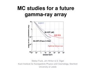
MC studies for a future gamma-ray array. Stefan Funk, Jim Hinton & S. Digel Kavli Institute for Astroparticle Physics and Cosmology, Stanford University of Leeds. Outline. Part 1: Angular resolution MC-studies Part 2: Toy MC for fast exploration of phase space

E N D
MC studies for a future gamma-ray array Stefan Funk, Jim Hinton & S. Digel Kavli Institute for Astroparticle Physics and Cosmology, Stanford University of Leeds
Outline • Part 1: Angular resolution MC-studies • Part 2: Toy MC for fast exploration of phase space • Part 3: The high-energy part of the array • Part 4: Simulated Survey
Angular resolution studies • Can be well studied with simple -ray MCs (no need for Hadrons) • One of the main drivers for any design study • Simplified telescope simulation • Corsika 6.204, simulate -rays • Record cherenkov photons • Atmospheric transmission, QE, mirror reflectivity, night-sky BG • Assume perfect optics • Minimisation of shower axis (core position and direction) in all images simultaneously • Variables are: • pixel size, fov, … • array spacing, dish size, …
First step: reproduce HESS • For H.E.S.S.-style telescopes, i.e. • 4 telescopes, • 0.14 deg pixels • 5 deg FoV • 11.8 m dish diameter • Size-cut 200 • … • Get something that matches H.E.S.S.
Second step: try to get something close to the optimal resolution • Something like: • 49 telescopes • Pixel size 0.06 deg • Seperation: 50 m • Dish-diameter: 30 m • … • Somehow the biggest things we could come up with • About a factor 2 worse than Werner’s curve (0.02° 68%-containment-2D at 1 TeV)
Now investigate several effects • So-called reference array: • 25 telescopes • 100 m spacing • Pixel size 0.08° • 15m dish diameter • 6° FoV • Gate width: 32 ns • Investigate effects of: • Pixel size • Telescope multiplicity • Dish diameter • FoV • Telescope spacing, …
Angular resolution vs pixelsize • For reference array • Keep the FoV constant (at 6º) and change the pixel size • Might be unrealistic (just increases the number of pixels as pixel size decreases) • Therefore try with fixed number of pixels (36x36) and adjust the field of view as the pixel size changes … • Also no strong dependence on pixel size (different with different reconstruction algorithm?) • … and FoV only matters if very small (1.44º for pix size 0.04º)
Angular resolution vs multiplicity • Started with array of 49 telescopes (distance: 100 m) • randomly kept 9, 16, 25, 36, 49 telescopes • Angular resolution vs average multiplicity • No strong dependence on any of the other tested parameters … (FoV, mirror size, …)
Use these finding to parametrise the curves … Mostly by J. Hinton J68 0.02 (E / TeV)0.62 ( (0.09/Ntels)2 + (0.17/<image_size>1/2)2 )1/2 degrees • Explore the dependence of • angular resolution • hadron rejection power • … on key factors such as: • Telescope multiplicity • Average size (in p.e.) of images • the impact distance range of the measurements • the pixel size (All as a function of energy) • Critical inputs to the Toy MC as discussed in the next slides …
… and then use them as input for the toy MC Mostly by J. Hinton • Driven by the need to explore the (rather large) phase-space • Full MC takes a LONG time to assess one configuration – how can we optimise the array? • Using an approximate Toy MC we can explore (orders of magnitude) more of the phase space and find plausible candidate array layouts to simulate in detail • BUT: • This is only useful if the Toy MC has realistic inputs and has real predictive power
Inputs to the Toy model • Only Vertical showers • Cherenkov Light Density (r, E) [ LDF ] • Displacement of image with impact distance • Fluctuations: Xmax, E, and Poisson in image Effective Area Curves Gamma-ray rate (E) • Background rate? • Electron and Proton spectra • Angular resolution parameterisation • Versus <size> and <Ntels> • BG rejection eff. parameterisation • Versus <size> and <Ntels> • Sensitivity (E) e.g. 200 GeV photoelectrons/m2/GeV Impact distance (m) Taken from de la Calle & Perez (2006)
Results: e.g. H.E.S.S. • 4 telescopes • 11.6 m diameter • 4.8 deg FoV • 4.6 million euro nominal cost • Core positions of triggering showers: (weighted to E-2 spectrum) • Effective area: effectively a post-cut area (edge cut, image size cut) • Also store <Ntel>(E) and <size>(E) • 10000 showers per energy bin 5 seconds total CPU
Resulting H.E.S.S. sensitivity Integral: E*Fmin(>E) Differential: half decades >10 gs BG limited full HE.S.S. MC
Resulting AGIS/CTA sensitivity • Bernloehr-style array (85 + 4 telescopes) • Can be reproduced quite well with the toy MC … Toy HESS full MC (KB)
280 m, 6.5 deg Optimisation for a grid … • Cost is fixed ($ 100M) • Number of tels varies • Free parameters • FoV • Telescope separation • Dish size • Pixel size kept fixed for the moment • Key input is missing (effect on hadron rejection of pixel size) • Grid search in 2-D planes within 3-D space … Example: HESS type array, optimise separation. • For a Crab-like spectrum and point-like source Photons cm-2 s-1 (>1 TeV) 180 60 m Telescope Separation (m)
Some thoughts on hybrid arrays 4x20m diam, 6.5° FoV, 0.1° pixels (Low E array) 19x12m diam, 7.5° FoV, 0.18° pixels (Prec. array) 21x12m diam, 10° FoV, 0.3° pixels (Large area array) • Aim: wide energy coverage • Optimising on a power-law tends to result in thresholds >= 100 GeV • Possible strategy • Optimise half(?) of budget on “pulsar-type spectrum” • (120 m sep, 20m telescopes, 5 deg FoV ) • Other half on power-law • ( 300 m sep, 10 m telescopes, 7.5 deg FoV ) • Then merge arrays? • Otherwise – optimise directly on “sensitive spectral coverage” – something like: • Integral over E of log(0.01*F(Crab)/Fmin) * dlogE ? • Or just FCrab(E)/Fmin(E) dlogE Same, but with more smaller Telescopes in the outskirts
Resulting Sensitivities • Quite promising to achieve design goals of energy coverage within budget
Summary for Toy Studies Mostly by J. Hinton • Next steps: • Need better input on hadron rejection performance • Need to add dependence of resolution and rejection power on pixel size • “Full” phase space exploration??? • Telescope diameter • FoV • Pixel size • Telescope separation • Island separation • Telescopes per island • *3 + fraction of budget on each part (3) • 21 dimensional search???
Part 3: The high-energy part of the array • How would one design an optimal array for the highest energies? • In terms of angular resolution and optimal coverage for 20-100 TeV region • Requirements: • Small dishes, large FoV, largish pixels … very relaxed requirements (lots of light!) • How large? Will answer this with our simulations … • Could easily surpass existing arrays where we are limited by the small FoV … • … more to come on this rather soon!
Together with J. Hinton and S. Digel Part 4: The simulated survey • Using H.E.S.S. backgrounds and a source population model to predict the outcome of a Galactic plane survey with a future instrument • E.g.: factor 10 better sensitivity • Factor 10 larger area • Factor 2 better PSF • Factor 2 better background rejection HESS : ~500 hours
The ‘Galactic plane with a future TeV instrument • Background: • Take H.E.S.S. survey data • Replace data with photons randomly sampled from the acceptance function (number of gamma-ray-like events versus camera offset - excluding source regions) taking into account zenith-dependence • This gives a “source-free” simulation of the HESS survey • Includes realistic exposure times and exactly the same analysis scheme as for the ‘real’ HESS survey ‘HESS - no sources’ : ~500 hours
The ‘Galactic plane with a future TeV instrument • Sources: • Take population model like in survey paper that matches H.E.S.S. properties: • Galactic latitude distribution • Source size distribution • Flux distribution • Different Populations: • SNRs: • Radial distribution of SNRs in Galaxy (Case & Bhattacharya A&AS120 p437 (1996)) • SNR explosion energies(Sveshnikova, 2003) • Source sizes from Sedov solution • PWNe: • Positions + energies from ATNF • Source evolution taken from H.E.S.S. sources • E.g. SNRs: -ray emission calculated based on DAV (Drury, Aharonian, Voelk 1996) from parameters such as Esn, , nmedium • Esn: SN explosion energy • : efficiency into gamma-rays • nmedium: density of surrounding medium
Matching H.E.S.S. • Need smallish scale height (30pc) to match narrow H.E.S.S. distribution • Rather normal efficiency into -rays: 9% • About 10 SNRs per century • … yields very good agreement (putting in H.E.S.S. source parameters, not source model)
Going beyond H.E.S.S. … • H.E.S.S. exposure rather uneven. Cut at 5 hours max at each point on the plane to get flat exposure • Increase area by factor 10, background rejection by factor 2, angular resolution by factor 2 (overall factor ~ 9) • Model predict ~ 150-500 sources within l= ±30°
Going beyond H.E.S.S. … • H.E.S.S. exposure rather uneven. Cut at 5 hours max at each point on the plane to get flat exposure • Increase area by factor 10, background rejection by factor 2, angular resolution by factor 2 (overall factor ~ 9) • Model predict ~ 150-500 sources within l= ±30°
Next steps • Do more than just pretty pictures. Nice playground for testing: • Source confusion • Trade-off between large area and good angular resolution • Energy dependent diffusion in the Galactic centre • ….
Summary • Simple MC to determine main dependencies of angular resolution • Combined with Toy MC to explore phase space • Working on characterisation of high-energy array • The simulated survey is a nice playground for testing physics questions