Extreme and smooth gradient percolation
700 likes | 973 Vues
Extreme and smooth gradient percolation. Bernard Sapoval Ecole polytechnique. Subtitle:. Fractal exponents (like 7/4) without fractals and without SLE and critical fluctuations without critical parameter. Agnès Desolneux (MAP 5, Université Paris 5)

Extreme and smooth gradient percolation
E N D
Presentation Transcript
Extreme and smooth gradient percolation Bernard Sapoval Ecole polytechnique
Subtitle: Fractal exponents (like 7/4) without fractals and without SLE and critical fluctuations without critical parameter Agnès Desolneux (MAP 5, Université Paris 5) Andrea Baldassarri (Università La Sapienza, Roma)
Diffuse distribution of particles on a lattice: gradient percolation Particles source Lg Lg+1 lines Particles sink L columns
Smooth gradient percolation: At each occupied site a continuous gaussian distribution with a variance s2 is attached. F(x,y) =(1/2s2)occup. sites iexp-{[(x-xi)2 +(y-yi)2] / 2s2} Then the contributions of the occupied sites are summed:
The contributions of the occupied sites are summed: 500 x 500 s = 2
Find the constant level lines: Whatever the level, one observes similar fluctuations. Critical fluctuations but around an arbitrary level
Physical problems at the origin of gradient percolation: • Diffusion fronts: geometry of diffuse contacts and soldering. • Structure of fuzzy images. • Corrosion fronts in the etching of random solids. • Erosion fronts: sea-coasts geometry.
DIFFUSE STRUCTURE: • The front is characterized by • its position xf , • itswidthf • and its lengthNf. Lg 2
A source of particles is kept at a constant concentration =1 At time t > 0, the particle concentration at a distance x is given by the complementary error function: is the diffusion length at time t where
If nf(x) is the mean number per unit horizontal length of points of the front:
Diffusion fronts: geometry of diffuse contacts and soldering.
What is gradient percolation? Random distribution of particles with a gradient of concentration. ≈ Lg4/7 The gradient percolation front is the frontier of the infinite cluster Mathematical aspects: P. Nolin
Numerical observations The average front position is such that, for large Lg, p(xf) is close to pc pc = 0.59280 ± 10-5 Rosso, Gouyet, BS(1985) pc = 0.592745 ± 2. 10-6 Ziff, BS (1986) pc = 0.5927460 ± 5. 10-7 Ziff and Stell (1988)
First measurements of the front fractal dimension… Df = 1.76 ± 0.02. (1984)
1984 The front width f followed a power law f Lgwith ≈ 0.57… The front length Nf followed a power law Nf Lgwith ≈ 0.42…
An island is a finite cluster because it is situated at a position x where p(x) < pc = 4/3 (den Nijs, 1983) = 0.5714…
Front length Nf: The front widthbeing acorrelation length: Nf is of order (L/ ).Df Lg 2 • Nf ≈ L.(Df-1) ≈L. Lg = (Df-1)/(1 + ) ≈ 0.426 The fact thatis the horizontal correlation length has been shown recently by Pierre Nolin (arXiv:math/0610682)
but one had + ≈ 1 /(1 + ) + (Df-1)/(1 + ) = 1 Df=(1+ )/ Df / (1+ ) ≈ 1 Df=7/4 ??? Percolation cluster hull conjecture (1984)
But now we know (Duplantier, 1987, Smirnov, 2001) that for sure Df = 7/4: The number of particles in a box of lateral width is :(Nf/L). ≈ Df ≈ Lg Df . / (1+ ) ≈Lg • But (Nf/L).is the number of particles in a box of sizewhere is the statistical width of the frontier. This width is defined independently of the fractal character of the frontier. Fractality does not appear in this statement
For diffusion, it means that the correlated surface is of the order of the diffusion length at time t:lD(t) = 2(Dt)1/2
What if the gradient is so large that the frontier is no more fractal? Small Lg values? The same power laws are observed
Statistique des fractures: empirique ou théorique? Attaque corrosif d’une couche mince d'aluminium plongé dans une solution Expériences: L.Balazs (1996) PMC Ecole Polytechnique. CCD Camera Aluminium Solution Verre Lumière
Other situation with gradient percolation: pit corrosion of an aluminum film. L. Balasz (Ecole polytechnique,1997)
Time evolution of the corrosion picture: • The first circular pit grows with time. • It roughens progressively and slows down. • It finally stops on a fractal frontier with dimension 4/3.
The corrosion model: • Andrea Baldassari • Andrea Gabrielli
Width of the front as a function of the gradient but where is the gradient?
Rocky coast-line erosion has marine and atmospheric causes which act on random ‘lithologic’units: random rocksRandom means that the ‘mechano-chemical’ properties of the rocks (due to structure and composition) are unknown and exhibit some dispersion. • EROSION OF ROCKY COASTS:
Sea-coasts could be fractal because their geometry damps the sea-waves (and currents …) in such manner that, for a given ‘sea power ’, the erosion is minimized. In that sense it is not only the coast which is erodedbut the effective erosion force of the sea which is diminished by the geometry of the coast.And this is why one observes fractal sea-coasts ????Phys. Rev. Lett. 2004.http://www.nature.com/nsu/031124/031124-4.html
The sea power and erosion force is a decreasing function of the coast perimeter, for example: g
The ‘resisting’ earth is represented by a square lattice where each site presents a random lithology or resistance to the sea. x11 x12 x13 x14 x15 x6 x7 x8 x9 x10 x1 x2 x3 x4 x5
x11 x12 x13 x14 x15 x11 x12 x13 x14 x15 x6 x7 x8 x9 x10 x6 x7 x8 x10 x1 x3 x5 x1 x3 x5 Lp = 5 , f(t=1) = f(t=0) Lp = 7 , f(t=2) < f(t=0) x11 x12 x13 x14 x15 x6 x7 x8 x9 x10 x1 x2 x3 x4 x5 Lp = 5 , f(t=0) Model representation of the erosion process The weaker sites are eroded and, at the same time: 1- new sites (strong or weak) are uncovered. 2- the coastal length is modified.
Time evolution: fractal morphology is a statistical geometrical attractor
North Sardinia real and numerical Df, num. = 4/3 Df, geo. = 1.33
Box-counting determination of the fractal dimension The value 4/3 is the dimension of the percolation cluster accessible perimeter. (Grossman, Aharony, 1985) (Duplantier et al. 1999) Df = 4/3
Scaling behavior of the coast width 4/7 is related to gradient percolation
The erosion model in itself is more general. It could apply to rough but non-fractal coastline:
What if the gradient is so large that the frontier is no more fractal? Small Lg values? The same power laws are observed
Extreme gradient percolation or fractal exponents without fractals • A. DESOLNEUX, B. SAPOVAL, and A. BALDASSARRI, • Self-Organised Percolation Power Laws with and without Fractal Geometry in the Etching of Random Solids, • in “Fractal Geometry and Applications” • Proceedings of Symposia in Pure Mathematics (PSPUM). • American Mathematical Society • In print. Seecond-mat/0302072.
Note that if percolation had been defined in the first place through gradient percolation :…. pc = 1/2
Remark: for small Lg • One expects a law of the form 7/4 = a(Lg+ b) And Nf7/3= c(Lg+ d) Is b = -1?
Numerical test of the exponent: Is 7/4 the best exponent? 1- Choose arbitrary 1.6 < a < 1.9. 2- Find the best fit values of the law sa = aa(Lg+ ba). 3- Then for each a, compute the distance:
Result: d(a)2 a