Download
1 / 27
270 likes | 423 Vues
Introduction to Transfer Learning (Part 2) For 2012 Dragon Star Lectures. Qiang Yang Hong Kong University of Science and Technology Hong Kong, China http:// www.cse.ust.hk/~qyang. Domain Adaptation in NLP. Applications. Selected Methods.

E N D
Introduction to Transfer Learning (Part 2) For 2012 Dragon Star Lectures Qiang Yang Hong Kong University of Science and Technology Hong Kong, China http://www.cse.ust.hk/~qyang
Domain Adaptation in NLP Applications Selected Methods Domain adaptation for statistical classifiers [Hal Daume III & Daniel Marcu, JAIR 2006], [Jiang and Zhai, ACL 2007] Structural Correspondence Learning [John Blitzer et al. ACL 2007] [Ando and Zhang, JMLR 2005] Latent subspace [SinnoJialin Pan et al. AAAI 08] • Automatic Content Extraction • Sentiment Classification • Part-Of-Speech Tagging • NER • Question Answering • Classification • Clustering
Instance-transfer Approaches[Wu and Dietterich ICML-04] [J.Jiang and C. Zhai, ACL 2007] [Dai, Yang et al. ICML-07] • Cross-domain POS tagging, • entity type classification • Personalized spam filtering Correct the decision boundary by re-weighting Uniform weights Loss function on the target domain data Loss function on the source domain data Regularization term • Differentiate the cost for misclassification of the target and source data
AdaBoost [Freund et al. 1997] To decrease the weights of the misclassified data To increase the weights of the misclassified data Source domain labeled data The whole training data set target domain labeled data Hedge ( ) [Freund et al. 1997] Classifiers trained on re-weighted labeled data Target domain unlabeled data TrAdaBoost[Dai, Yang et al. ICML-07] • Misclassified examples: • increase the weights of the misclassified target data • decrease the weights of the misclassified source data Evaluation with 20NG: 22%8%http://people.csail.mit.edu/jrennie/20Newsgroups/
Locally Weighted Ensemble[Jing Gao, Wei Fan, Jing Jiang, Jiawei Han: Knowledge transfer via multiple model local structure mapping. KDD 2008] Training set 1 C1 Training set 2 C2 Test example …… …… Training set k Ck • Graph-based weights approximation • Weight of a model is proportional to the similarity between itsneighborhood graph and the clustering structure around x.
Transductive Transfer Learning Instance-transfer ApproachesSample Selection Bias / Covariance Shift[Zadrozny ICML-04, Schwaighofer JSPI-00] Input:A lot of labeled data in the source domain and no labeled data in the target domain. Output: Models for use in the target domain data. Assumption: The source domain and target domain are the same. In addition, and are the same while and may be different caused by different sampling process (training data and test data). Main Idea: Re-weighting (important sampling) the source domain data.
Sample Selection Bias/Covariance Shift To correct sample selection bias: How to estimate ? One straightforward solution is to estimate and , respectively. However, estimating density function is a hard problem. weights for source domain data
Sample Selection Bias/Covariance ShiftKernel Mean Match (KMM)[Huang et al. NIPS 2006] Main Idea:KMM tries to estimate directly instead of estimating density function. It can be proved that can be estimated by solving the following quadratic programming (QP) optimization problem. Theoretical Support: Maximum Mean Discrepancy (MMD) [Borgwardt et al. BIOINFOMATICS-06]. The distance of distributions can be measured by Euclid distance of their mean vectors in a RKHS. To match means between training and test data in a RKHS
Feature Space: Document-word co-occurrence Source D_S Knowledge transfer D_T Target
Co-Clustering based Classification (KDD 2007) • Co-clustering is applied between features (words) and target-domain documents • Word clustering is constrained by the labels of in-domain (Old) documents • The word clustering part in both domains serve as a bridge 10
Structural Correspondence Learning [Blitzer et al. ACL 2007] • SCL: [Ando and Zhang, JMLR 2005] • Define pivot features: common in two domains • Build Latent Space built from Pivot Features, and do mapping • Build classifiers through the non-pivot Features
SCL[Blitzer et al. EMNLP-06, Blitzer et al. ACL-07, Ando and Zhang JMLR-05] a) Heuristically choose m pivot features, which is task specific. b) Transform each vector of pivot feature to a vector of binary values and then create corresponding prediction problem. Learn parameters of each prediction problem Do Eigen Decomposition on the matrix of parameters and learn the linear mapping function. Use the learnt mapping function to construct new features and train classifiers onto the new representations. Courtesy of Sinno Pan
Self-Taught Learning Feature-representation-transfer ApproachesUnsupervised Feature Construction[Raina et al. ICML-07] Three steps: • Applying sparse coding[Lee et al. NIPS-07] algorithm to learn higher-level representation from unlabeled data in the source domain. • Transforming the target data to new representations by new bases learnt in the first step. • Traditional discriminative models can be applied on new representations of the target data with corresponding labels. Courtesy of Sinno Pan
Unsupervised Feature Construction[Raina et al. ICML-07] Step1: Input:Source domain data and coefficient Output:New representations of the source domain data and new bases Step2: Input:Target domain data , coefficient and bases Output:New representations of the target domain data Courtesy of Sinno Pan
“Self-taught Learning”[Raina et al. Self-Taught Learning ICML-07] + ? Labeled Webpages Labeled Digits Unlabeled English characters + ? Unlabeled newspaper articles + ? Unlabeled English speech Labeled Russian Speech Self-taught Learning: Courtesy of Raina
Examples of Higher Level Features Learned Learnt bases: “Edges” Natural images. Learnt bases: “Strokes” Handwritten characters. Self-taught Learning: Courtesy of Raina
Latent Feature Space TL Methods: Temporal Domain Distribution Changes The mapping function f learned in the offline phase can beout of date. Recollecting the WiFi data is very expensive. How to adapt the model ? Time Night time period Day time period
Transfer Component Analysis: SinnoPan et al., IEEE Trans. NN 2011 If two domains are related, … Observations Source Domain data Target Domain data Latent factors Common latent factors across domains SinnoJialin Pan
Motivation (cont.) Observations Source domain data Target domain data Latent factors • Some latent factors may preserve important properties (such as variance, local topological structure) of the original data, while others may not. SinnoJialin Pan
PCA: Only Maximizing the Data Variance Principal Component Analysis (PCA) [Jolliffe. 02] aims to find a low-dimensional latent space where the variance of the projected data is maximized. Con: it may not reduce the difference between domains. SinnoJialin Pan
Learning the Transform Mapping High level optimization problem • How to estimate distance between distributions in the latent space? • How to solve the resultant optimization problem? SinnoJialin Pan
Semi-Supervised TCA To measure the distance between domains using MMD High level objectives: To measure label dependence using Hilbert-Schmidt Independence Criterion (HSIC) SinnoJialin Pan
Blitzer, et al. Learning Bounds for Domain Adaptation. NIPS 2007 m’=number of examples d(u_S, u_T) = domain distance 1-d=confidence e=error
Inductive Transfer LearningModel-transfer ApproachesRegularization-based Method[Evgeiou and Pontil, KDD-04] Assumption: If t tasks are related to each other, then they may share some parameters among individual models. Assume be a hyper-plane for task , where and Encode them into SVMs: Common part Specific part for individual task Regularization terms for multiple tasks
Inductive Transfer LearningStructural-transfer ApproachesTAMAR[Mihalkova et al. AAAI-07] Assumption: If the target domain and source domain are related, then there may be some relationship between domains that are similar, which can be used for transfer learning Input: • Relational data in the source domain and a statistical relational model, Markov Logic Network (MLN), which has been learnt in the source domain. • Relational data in the target domain. Output: A new statistical relational model, MLN, in the target domain. Goal: To learn a MLN in the target domain more efficiently and effectively.
TAMAR [Mihalkova et al. AAAI-07] Two Stages: • Predicate Mapping • Establish the mapping between predicates in the source and target domain. Once a mapping is established, clauses from the source domain can be translated into the target domain. • Revising the Mapped Structure • The clause-mapping from the source domain directly may not be completely accurate and may need to be revised, augmented , and re-weighted in order to properly model the target data.
Actor(A) Director(B) WorkedFor Student (B) Professor (A) AdvisedBy MovieMember MovieMember Movie(M) Publication Publication Paper (T) TAMAR [Mihalkova et al. AAAI-07] Source domain (academic domain) Target domain (movie domain) Mapping Revising