Download
1 / 17
170 likes | 315 Vues
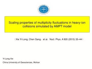
Scaling properties of multiplicity fluctuations in heavy-ion collisions simulated by AMPT model. ( Xie Yi-Long, Chen Gang , et al , Nucl. Phys. A 920 (2013) 33–44 ). Yi-Long Xie China University of Geosciences, Wuhan. Content. Nonlinear Dynamics AMPT model Results of NFM Analysis

E N D
Scaling properties of multiplicity fluctuations in heavy-ion collisions simulated by AMPT model (Xie Yi-Long, Chen Gang,et al,Nucl. Phys. A 920 (2013) 33–44) Yi-Long Xie China University of Geosciences, Wuhan
Content Nonlinear Dynamics AMPT model Results of NFM Analysis Discussion of FM’s Scaling Summary China University of Geosciences School of mathematics and physics
1. Nonlinear Dynamics China University of Geosciences School of mathematics and physics Big local fluctuation implied dynamical factors. Bialas:describe the fluctuation with NFM as follow:
1. Nonlinear Dynamics China University of Geosciences School of mathematics and physics Criterion for existence of fractal Self-similar Fractal Self-affine Fractal
1. Nonlinear Dynamics China University of Geosciences School of mathematics and physics Characterize of Self-similar Fractal: Isotropicpartition the phase-space Characterize of Self-affine Fractal Anisotropic partition the phase-spacewith calculatedHurst exponent Fitting the 1-d NFM with saturation exponents Calculate the Hurst exponent with saturation exponent Wu Y F, Liu L S. Phys Rev Lett, 1993, 70(21):3197-3200
1. Nonlinear Dynamics China University of Geosciences School of mathematics and physics Self-similar Fractal Self-affine Fractal collision at region Hadron collision Abreu P, Adam W, Adye T, et al. Nucl Phys B, 1992, 386(2):471-492 Agababyan N M, Atayan M R, Charlet M, et al. Phys Lett B, 1996, 382(3):305-311
1. Nonlinear Dynamics China University of Geosciences School of mathematics and physics Experiments has shown that: The final state system in hadron collisions is self-affine fractal The final state system in collisions at region is self-affine fractal So: Does fractal exist in heavy ion collisions? Which kind of fractal?
2 AMPT model A Pictorial View of Micro-Bangs at RHIC: 1. Initial Condition 2. Partonic Cascade 3. Hadronization 4. Hadronic Rescattering
2 AMPT model (a) AMPT v1.11 (Default) (b) AMPT v2.11 (String Melting)
3.1 Results of NFM Analysis Fig.1. 1-D NFM: (q=2). China University of Geosciences School of mathematics and physics 1. 1-D NFM tends to saturate 2. Saturation exponents: 3. Identical Hurst exponents: Tab.1. Fitting parameters for 1-D NFM (q=2).
3.2 Results of NFM Analysis China University of Geosciences School of mathematics and physics Fig.2. The logarithm distribution of 2-D NFM, i.e. Fitting formula: Show good Scaling Conclusion: Self-Similar Fractal
3.3 Results of NFM Analysis China University of Geosciences School of mathematics and physics • Fitting Formula: • Same Conclusion: Scaling Featureand Self-similar Fractal 2. Fluctuation in heavy ion collision is larger than those in hadron collisions and collisions. Effect Fluctuation Strength: QGP Fig.3. The logarithm distribution of 3-D NFM: Tab.3. Effect Fluctuation Strength Tab.2. Fitting parameter for 3-D NFM
4. Discussion of FM’s Scaling China University of Geosciences School of mathematics and physics RudophC. Hwa, M. T. Nazirov, Phys. Rev. Lett. 69 (1992) 1741. Fig.4. The distribution of 3-D NFM: Fig.5. Parameter are obtained when fitting the relation: Fitting Formula: Fitting Formula: Scaling property is checked again. • . Not phase transition in AMPT.
4. Discussion of FM’s Scaling China University of Geosciences School of mathematics and physics Fig.6. The loglog distribution of 2-D NFM in the plane at various intervals • Expectation: • Indeed, Fluctuation with 3. Due to the limited events, quantitative analysis can’t be made.
4. Discussion of FM’s Scaling Fluctuation in high is actually much larger than that in low . Fig.7. The distribution of 2-D NFM as a function of , with partition number M=1 2D FM on plane(M=1): China University of Geosciences School of mathematics and physics rapidly with .
5 Summary China University of Geosciences School of mathematics and physics 1. With the data of Au-Au collision events at 200Gev generated by AMPT model, the 1-D NFM is obtained. The obtained Hurst exponent approximately equal to 1 within the error range. 2. Partitioning the phase-space according to Hurst exponent, then calculate the 2-D and 3-D NFMs. They both show good scaling, which means the final state system is self-similar fractal. 3. According to the calculated effect fluctuation strengths, the fluctuation in heavy ion collisions is found to be much smaller than those in hadron-hadron collisions and electron-positron collisions, which may be the signal of QGP. 4. When checking the scaling property again, the parameter can be obtained. Our results is larger than v =1.304 derived in Ginzburg-Landau type of phase transition. AMPT does not include the phase transition. 5. Splitting the pt range into smaller intervals, the in high is expected to be larger than that in low . Due to the limited events, quantitative analysis can’t be made. But if considering the 2D FM on (M=1), we actually see the increasing of fluctuation with the increasing of pt.