Review on Linear Algebra
Review on Linear Algebra. Contents. Introduction to System of Linear Equations, Matrices, and Matrix Operations Euclidean Vector Spaces General Vector Spaces Inner Product Spaces Eigenvalue and Eigenvector. Introduction to System of Linear Equations, Matrices, and Matrix Operations.

Review on Linear Algebra
E N D
Presentation Transcript
Contents • Introduction to System of Linear Equations, Matrices, and Matrix Operations • Euclidean Vector Spaces • General Vector Spaces • Inner Product Spaces • Eigenvalue and Eigenvector
Introduction to System of Linear Equations, Matrices, and Matrix Operations
Linear Equations • Any straight line in xy-plane can be represented algebraically by an equation of the form: a1x + a2y = b • General form: Define a linear equation in the n variables x1, x2, …, xn : a1x1 + a2x2 + ··· + anxn = b where a1, a2, …, an and b are real constants. • The variables in a linear equation are sometimes called unknowns.
Example (Linear Equations) • The equations andare linear • A linear equation does not involve any products or roots of variables • All variables occur only to the first power and do not appear as arguments for trigonometric, logarithmic, or exponential functions. • The equations are not linear (non-linear)
Example (Linear Equations) • A solution of a linear equation is a sequence of n numbers s1, s2, …, sn such that the equation is satisfied. • The set of all solutions of the equation is called its solution set or general solution of the equation.
Linear Systems • A finite set of linear equations in the variables x1, x2, …, xn is called a system of linear equations or a linear system. • A sequence of numbers s1, s2, …, sn is called a solution of the system • A system has no solution is said to be inconsistent. • If there is at least one solution of the system, it is called consistent. • Every system of linear equations has either no solutions, exactly one solution, or infinitely many solutions
Augmented Matrices • The location of the +s, the xs, and the =s can be abbreviated by writing only the rectangular array of numbers. • This is called the augmented matrix (擴增矩陣) for the system. • It must be written in the same order in each equation as the unknowns and the constants must be on the right
In computer science an array is a data structure consisting of a group of elements that are accessed by indexing. 1st column 1st row Augmented Matrices • It must be written in the same order in each equation as the unknowns and the constants must be on the right Matrix
Homogeneous(齊次) Linear Systems • A system of linear equations is said to be homogeneous if the constant terms are all zero; that is, the system has the form:
Homogeneous Linear Systems • Every homogeneous system of linear equation is consistent, since all such system have x1 = 0, x2 = 0, …, xn = 0 as a solution. • This solution is called the trivial solution(零解). • If there are another solutions, they are called nontrivial solutions(非零解). • There are only two possibilities for its solutions: • There is only the trivial solution • There are infinitely many solutions in addition to the trivial solution
Theorem • Theorem 1 • A homogeneous system of linear equations with more unknowns than equations has infinitely many solutions. • Remark • This theorem applies only to homogeneous system! • A nonhomogeneous system with more unknowns than equations need not be consistent; however, if the system is consistent, it will have infinitely many solutions. • e.g., two parallel planes in 3-space
Definition and Notation • A matrix is a rectangular array of numbers. The numbers in the array are called the entries in the matrix • A general mn matrix A is denoted as
Definition and Notation • The entry that occurs in row i and column j of matrix A will be denoted aij or Aij. If aij is real number, it is common to be referred as scalars • The preceding matrix can be written as [aij]mn or [aij] • A matrix A with n rows and n columns is called a square matrix of order n
Definition • Two matrices are defined to be equal if they have the same size and their corresponding entries are equal • If A = [aij] and B = [bij] have the same size, then A = B if and only if aij = bij for all i and j • If A and B are matrices of the same size, then the sumA + B is the matrix obtained by adding the entries of B to the corresponding entries of A.
Definition • The differenceA – B is the matrix obtained by subtracting the entries of B from the corresponding entries of A • If A is any matrix and c is any scalar, then the productcA is the matrix obtained by multiplying each entry of the matrix A by c. The matrix cA is said to be the scalar multiple of A • If A = [aij], then cAij = cAij = caij
Definitions • If A is an mr matrix and B is an rn matrix, then the productAB is the mn matrix whose entries are determined as follows. • To find the entry in row i and column j of AB, single out row i from the matrix A and column j from the matrix B. Multiply the corresponding entries from the row and column together and then add up the resulting products
Definitions • That is, (AB)mn = Amr Brn the entry ABij in row i and column j of AB is given by ABij = ai1b1j+ ai2b2j + ai3b3j + … + airbrj
Partitioned Matrices • A matrix can be subdivided or partitionedinto smaller matrices by inserting horizontal and vertical rules between selected rows and columns
Partitioned Matrices • For example, three possible partitions of a 34 matrix A: • The partition of A into four submatricesA11, A12, A21, and A22 • The partition of A into its row matrices r1, r2, and r3 • The partition of A into its column matrices c1, c2, c3, and c4
Multiplication by Columns and by Rows • It is possible to compute a particular row or column of a matrix product AB without computing the entire product: jth column matrix of AB = A[jth column matrix of B] ith row matrix of AB = [ith row matrix of A]B
Multiplication by Columns and by Rows • If a1, a2, ..., am denote the row matrices of A and b1 ,b2, ...,bn denote the column matrices of B, then
Matrix Products as Linear Combinations • Let • Then • The product Ax of a matrix A with a column matrix x is a linear combination of the column matrices of A with the coefficients coming from the matrix x
Matrix Form of a Linear System • Consider any system of m linear equations in n unknowns: • The matrix A is called the coefficient matrix of the system • The augmented matrix of the system is given by
Definitions • If A is any mn matrix, then the transpose of A, denoted by AT, is defined to be the nm matrix that results from interchanging the rows and columns of A • That is, the first column of AT is the first row of A, the second column of AT is the second row of A, and so forth
Definitions • If A is a square matrix, then the trace of A , denoted by tr(A), is defined to be the sum of the entries on the main diagonal of A. The trace of A is undefined if A is not a square matrix. • For an nn matrix A = [aij],
Properties of Matrix Operations • For real numbers a and b ,we always have ab = ba, which is called the commutative law for multiplication. For matrices, however, AB and BA need not be equal. • Equality can fail to hold for three reasons: • The product AB is defined but BA is undefined. • AB and BA are both defined but have different sizes. • It is possible to have AB BA even if both AB and BA are defined and have the same size.
Theorem 2 (Properties of Matrix Arithmetic) • Assuming that the sizes of the matrices are such that the indicated operations can be performed, the following rules of matrix arithmetic are valid: • A + B = B + A (commutative law for addition) • A + (B + C) = (A + B) + C (associative law for addition) • A(BC) = (AB)C (associative law for multiplication) • A(B + C) = AB + AC (left distributive law) • (B + C)A = BA + CA (right distributive law) • A(B – C) = AB – AC, (B – C)A = BA – CA • a(B + C) = aB + aC, a(B – C) = aB – aC
Theorem 2 (Properties of Matrix Arithmetic) • (a+b)C = aC + bC, (a-b)C = aC – bC • a(bC) = (ab)C, a(BC) = (aB)C = B(aC)
Zero Matrices • A matrix, all of whose entries are zero, is called a zero matrix • A zero matrix will be denoted by 0 • If it is important to emphasize the size, we shall write 0mn for the mn zero matrix. • In keeping with our convention of using boldface symbols for matrices with one column, we will denote a zero matrix with one column by 0
Zero Matrices • Theorem 3 (Properties of Zero Matrices) • Assuming that the sizes of the matrices are such that the indicated operations can be performed ,the following rules of matrix arithmetic are valid • A + 0 = 0 + A = A • A – A = 0 • 0 – A = -A • A0 = 0; 0A = 0
Identity Matrices • A square matrix with 1s on the main diagonal and 0s off the main diagonal is called an identity matrixand is denoted by I, or In for the nn identity matrix • If A is an mn matrix, then AIn = A and ImA = A • An identity matrix plays the same role in matrix arithmetic as the number 1 plays in the numerical relationships a·1 = 1·a = a
Definition • If A is a square matrix, and if a matrix B of the same size can be found such that AB = BA = I, then A is said to be invertibleand B is called an inverseof A. If no such matrix B can be found, then A is said to be singular. • Remark: • The inverse of A is denoted as A-1 • Not every (square) matrix has an inverse • An inverse matrix has exactly one inverse
Theorems • Theorem 4 • If B and C are both inverses of the matrix A, then B = C • Theorem 5 • The matrix is invertible if ad – bc 0, in which case the inverse is given by the formula
Theorems • Theorem 6 • If A and B are invertible matrices of the same size ,then AB is invertible and (AB)-1 = B-1A-1
Definition • If A is a square matrix, then we define the nonnegative integer powers of A to be • If A is invertible, then we define the negative integer powers to be
Theorems • Theorem 7 (Laws of Exponents) • If A is a square matrix and r and s are integers, then ArAs = Ar+s, (Ar)s = Ars • Theorem 8 (Laws of Exponents) • If A is an invertible matrix, then: • A-1 is invertible and (A-1)-1 = A • An is invertible and (An)-1 = (A-1)n for n = 0, 1, 2, … • For any nonzero scalar k, the matrix kA is invertible and (kA)-1 = (1/k)A-1
Theorems • Theorem 9 (Properties of the Transpose) • If the sizes of the matrices are such that the stated operations can be performed, then • ((AT)T = A • (A + B)T = AT + BT and (A – B)T = AT – BT • (kA)T = kAT, where k is any scalar • (AB)T = BTAT • Theorem 10 (Invertibility of a Transpose) • If A is an invertible matrix, then AT is also invertible and (AT)-1 = (A-1)T
Theorems • Theorem 11 • Every system of linear equations has either no solutions, exactly one solution, or in finitely many solutions. • Theorem 12 • If A is an invertible nn matrix, then for each n1 matrix b, the system of equations Ax = b has exactly one solution, namely, x = A-1b.
Theorems • Theorem 13 • Let A be a square matrix • If B is a square matrix satisfying BA = I, then B = A-1 • If B is a square matrix satisfying AB = I, then B = A-1 • Theorem 14 • Let A and B be square matrices of the same size. If AB is invertible, then A and B must also be invertible.
Definitions • A square matrixA is mn with m = n; the (i,j)-entries for 1 i m form the main diagonal of A • A diagonal matrix is a square matrix all of whose entries not on the main diagonal equal zero. By diag(d1, …, dm) is meant the mm diagonal matrix whose (i,i)-entry equals di for 1 i m
Definitions • A mnlower-triangular matrixL satisfies (L)ij = 0 if i < j, for 1 i m and 1 j n • A mnupper-triangular matrixU satisfies (U)ij = 0 if i > j, for 1 i m and 1 j n • A unit-lower (or –upper)-triangular matrixT is a lower (or upper)-triangular matrix satisfying (T)ii = 1 for 1 i min(m,n)
A general nn diagonal matrix D can be written as A diagonal matrix is invertible if and only if all of its diagonal entries are nonzero Powers of diagonal matrices are easy to compute Properties of Diagonal Matrices
Properties of Diagonal Matrices • Matrix products that involve diagonal factors are especially easy to compute
Theorem 15 • The transpose of a lower triangular matrix is upper triangular, and the transpose of an upper triangular matrix is lower triangular • The product of lower triangular matrices is lower triangular, and the product of upper triangular matrices is upper triangular
Theorem 16 • A triangular matrix is invertible if and only if its diagonal entries are all nonzero • The inverse of an invertible lower triangular matrix is lower triangular, and the inverse of an invertible upper triangular matrix is upper triangular
Symmetric Matrices • Definition • A (square) matrix A for which AT = A, so that Aij = Aji for all i and j, is said to be symmetric. • Theorem 17 • If A and B are symmetric matrices with the same size, and if k is any scalar, then • AT is symmetric • A + B and A – B are symmetric • kA is symmetric
Symmetric Matrices • Remark • The product of two symmetric matrices is symmetric if and only if the matrices commute, i.e., AB = BA
Theorems • Theorem 18 • If A is an invertible symmetric matrix, then A-1 is symmetric. • Remark: • In general, a symmetric matrix needs not be invertible. • The products AAT and ATA are always symmetric