Hierarchical Well-Separated Trees (HST)

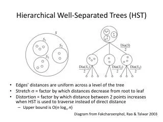
1. Hierarchical Well-Separated Trees (HST) • Edges’ distances are uniform across a level of the tree • Stretch s = factor by which distances decrease from root to leaf • Distortion = factor by which distance between 2 points increases when HST is used to traverse instead of direct distance • Upper bound is O(s logsn) Diagram from Fakcharoenphol, Rao & Talwar 2003

2. Pure Randomized vs. Fractional Algorithms • “Fractional view” = keep track only of marginal distributions of some quantities • Lossy compared to pure randomized • Which marginals to track? • Claim: for some algorithms, fractional view can be converted back to randomized algorithm with little loss

3. Fractional View of K-server Problem • For node j, let T(j) = leaves of the subtree of T rooted in j • At time step t, for leaf i, pit= probability of having a server at i • If there is a request at i on time t, pit should be 1 • Expected number of servers across T(j) = kt(j) = Si∈T(j)pit • Movement cost to get servers at j = Sj∈T W(j) |kt(j) – kt-1(j)| j T(j) i Parts of diagram from Bansal 2011

4. The Allocation Problem • Decide how to (re-)distribute k servers among d locations (each location of uniform distance from a center and may request arbitrary no. of servers) • Each location i has a request denoted as {ht(0), ht(1), … ht(k)} • ht(j) = cost of serving request using j servers • Ex.: request at i=0 is {∞, 2, 1, 0, 0} (monotonic decrease) • Total cost = hit cost + movement cost I can work with 1, but I’d like 3! Parts of diagram from Bansal 2011

5. Fractional View of Allocation Problem • Let xi,jt= (non-negative) probability of having j servers at location i at time t • Sum of probabilities Sjxi,jt = 1 • No. of servers used must not exceed no. available SiSjj ∙ xi,jt ≤ k • Hit cost incurred = Sjht(j) ∙ xi,jt • Movement cost incurred = Si Sj(|Sj’<jxi,jt– Sj’<jxi,jt-1|) • Note: fractional A.P. too weak to obtain randomized A.P. algorithm • But we don’t really care about A.P., we care about K-server problem!

6. From Allocation to K-Server • Theorem 2: It suffices to have a (1+, ())-competitive fractional APalgorithm on uniform metric to get a k-server algorithm that is O(βl)-competitive algorithm (Coté et al. 2008) • Theorem 1: Bansal et al.’s k-server algorithm has a competitive ratio of Õ(log2k log3n)

7. The Main Algorithm • Embed the n points into a distributionmover s-HSTs with stretch s = Q(log n log(k log n)) • (No time to discuss, this step is essentially from the paper of Fakcharoenphol, Rao & Talwar2003) • According to distribution m, pick a random HST T • Extra step: Transform the HST to a weighted HST (We’ll briefly touch on this) Diagram from Bansal 2011

8. The Main Algorithm • Solve the (fractional) allocation problem on T’s root node + immediate children, then recursively solve the same problem on each child • Intuitive application of Theorem 2 • d = immediate children of a given node • At root node: k = all k servers • At internal node i: k = resulting (re)allocation of servers from i’s parent Allocation instances Diagram from Bansal 2011

9. Detour: Weighted HST • Degenerate case of normal HST: • Depth l= O(n) (can happen if n points are on a line with geometrically increasing distances)

10. Detour: Weighted HST • Solution: allow lengths of edges to be non-uniform • Allow distortion from leaf-to-leaf to be at most 2s/(s–1) • Depth l = O(log n) • Consequence: Uniform A.P. becomes weighted-star A.P.

11. Proving the Main Algorithm • Theorem 1: Bansal et al.’s k-server algorithm has a competitive ratio of Õ(log2k log3n) • Idea of proof: How does competitive ratio and distortion evolveas we transform: Fractional allocation algorithm ↓ Fractional k-server algorithm on HST ↓ Randomized k-server algorithm on HST

12. Supplemental Theorems • Theorem 3: For e > 0, there exists a fractional A.P. algorithm on a weighted-star metric that is (1+e, O(log(k/e)))-competitive (Refinement of theorem 2, to be discussed by Tanvirul) • Theorem 4: If T is a weighted s-HST with depth l, if Theorem 3 holds, then there is a fractional k-server algorithm that is O(l log(kl))-competitive as long as s = W(l log(kl)) • Theorem 5: If T is a s-HST with s>5, then any fractional k-server algorithm on T converts to a randomized k-server algorithm on T that is about as competitive (only O(1) loss) • Theorem 6: If T is a s-HST with n leaves and any depth, it can transform to a weighted s-HST with identical leaves but with depth O(log n) and leaf-to-leaf distance distorted only by at most 2s/(s–1)

13. Proof of Theorem 1 • Embed the n points into a distributionm over s-HSTs with stretch s = Q(log n log(k log n)) • Distortion at O(s logsn) • Resulting HSTs may have depth l up to O(n) • According to distribution m, pick a random HST T and transform to a weighted HST • From Theorem 6, depth l reduced to O(log n) • Stretch s is now Q(l log (kl)))

14. Proof of Theorem 1 • Solve the (fractional) allocation problem on T’s root node + immediate children, then recursively solve the allocation problem on children • This is explicitly Theorem 2 refined by Theorem 3  • Stretch s =Q(l log (kl))), so Theorem 4 is applicable! • Transform to a fractional k-server algorithm with competitiveness = O(l log (kl))) = O(log n log (k log n)) • Applying Theorem 5, we get similar competitiveness for the randomized k-server algorithm

15. Proof of Theorem 1 • Expected distortion to optimal solution Opt*M, given the cost of the solution on T,cT: Em[cT] = O(s logsn) ∙ Opt*M AlgM≤ AlgT ≤ O(log n log (k log n)) ∙ cT Em[AlgM] = O(log n log (k log n)) ∙ Em[cT] = O(log n log (k log n)) ∙ O(s logsn) ∙ Opt*M

16. Proof of Theorem 1 Em[AlgM] = O(log n log (k log n)) ∙ O(s logsn) ∙ Opt*M • This implies a competitive ratio of: O(log n log (k log n)) ∙ O(s logsn) = O(log n log (k log n)) ∙O(s (log n / log s)) = O{[log3n (log (k log n))2] / log logn} = O(log2k log3n log logn) = Õ(log2k log3n)