Download
1 / 112
1.12k likes | 1.32k Vues
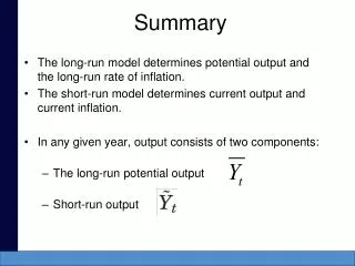
Summary. The long-run model determines potential output and the long-run rate of inflation. The short-run model determines current output and current inflation. In any given year, output consists of two components: The long-run potential output Short-run output. Short run output

E N D
Summary • The long-run model determines potential output and the long-run rate of inflation. • The short-run model determines current output and current inflation. • In any given year, output consists of two components: • The long-run potential output • Short-run output
Short run output • Is the percentage difference between actual and potential output. • Is positive when the economy is booming. • Is negative when the economy is slumping. • Recession: • Our Definition: • A period when actual output falls below potential • Short-run output becomes negative • (Ỹ < 0) • Usual Definition • (Roughly) 2 Quarters of negative GDP. • Declared by the NBER Business Cycle Dating Committee. • (ΔY < 0)
Short-run fluctuation • The difference in actual and potential output, expressed as a percentage of potential output • Referred to as “detrended output” or short-run output:
Ỹ < 0 Ȳ Ỹ < 0 ΔY<0 ΔY>0 ΔY<0 but Ỹ > 0 Recession Ends ΔY>0 but Ỹ < 0
A recession: • Begins when actual output falls below potential, and short-run output becomes negative. • Ends when short-run output starts to rise and become less negative. • During a recession: • Output is usually below potential for approximately two years, which results in a loss of about $2,400 per person. • Between 1.5 million and 3 million jobs are lost.
Measuring Potential Output • There is no directly observable measure of potential output in an economy. • Ways to measure potential output: • Assume a perfectly smooth trend passes through quarterly movements of real GDP. • Take averages of the surrounding actual GDP numbers.
9.3 The Short-Run Model • Short-run model features: • Open economy exists where global booms and recessions impact the local economy. • The economy will exhibit long-run growth and fluctuations. • Central Bank manages monetary policy to smooth fluctuations.
The short-run model is based on three premises: 1. The economy is constantly being hit by shocks: • Shocks: factors that cause fluctuations in output or inflation. 2. Monetary and fiscal policies affect output: • Policymakers may be able to neutralize shocks to the economy.
3. There is a dynamic trade-off between output and inflation: • The Phillips curve is the dynamic trade-off between output and inflation.
The Empirical Fit of the Phillips Curve • Empirically, the slope is approximately one-half. • Meaning: if output exceeds potential by 2 percent, the inflation rate increases one percentage point.
How the Short-Run Model Works • Assume policymakers can select short-run output through monetary policy • Example: • 1979: inflation was increasing because of oil prices • Monetary Policy: raise interest rates • What happens? • Recession!
Important thing about the Philip Curve • This is about accelerating and decelerating inflation. This is a change in the change of the price level • Is the Philips Curve fixed? • Supply Shocks. • Expectations.
Okun’s Law Cyclical unemployment Current rate of unemployment Short-run output Natural rate of unemployment
11.1 Introduction • In this chapter, we learn • The first building block of our short-run model: the IS curve • describes the effect of changes in the real interest rate on output in the short run. • How shocks to consumption, investment, government purchases, or net exports—“aggregate demand shocks”—can shift the IS curve.
A theory of consumption called the life-cycle/permanent-income hypothesis. • That investment is the key channel through which changes in real interest rates affect GDP in the short run.
The Federal Reserve exerts a substantial influence on the level of economic activity in the short run. • Sets the rate at which people borrow and lend in financial markets • The basic story is this:
The IS curve • The IS curve captures the relationship between interest rates and output in the short run. • There is a negative relationship between the interest rate and short-run output. • An increase in the interest rate will decrease investment, which will decrease output.
11.2 Setting Up the Economy • The national income accounting identity • Implies that the total resources available to the economy equal total uses • One equation with six unknowns Imports Production Investment Government purchases Exports Consumption
Consumption and Friends • Level of potential output is given exogenously. • Consumption C, government purchases G, exports EX, and imports IM depend on the economy’s potential output. • Each of these components of GDP is a constant fraction of potential output. • the fraction is a parameter
Potential output is smoother than actual GDP. • A shock to actual GDP will leave potential output unchanged • The equation depends on potential output. • Shocks to income are “smoothed” to keep consumption steady.
The Investment Equation A term weighting the difference between the real interest rate and the MPK Marginal Product of Capital (MPK) The share of potential output that goes to investment Real interest rate
The MPK • Is an exogenous parameter • Is time invariant • If the MPK is low relative to the real interest rate • Firms should save money and not invest in capital
If the MPK is high relative to the real interest rate • Firms should borrow and invest in capital • In the short run, the MPK and the real interest rate can be different. • Installing capital to equate the two takes time.
11.3 Deriving the IS Curve 1. Divide the national income accounting identity by potential output. 2. Substitute the five equations into this equation.
3. Recall the definition of short-run output. Simplifies the equation for the IS curve:
The gap between the real interest rate and the MPK is what matters for output fluctuations. • Firms can always earn the MPK on new investments. • The parameter • Is • Is called the aggregate demand shock • Will equal zero when potential output is equal to actual output
Case Study: Why is it called the “IS Curve”? • IS stands for “investment = savings” • See this again in Chapters 17 and 18.
11.4 Using the IS Curve The Basic IS Curve • When the demand shock parameter equals zero, the IS curve has a short-run output of 0 where the real interest rate is equal to the long-run value of the MPK.