Download
1 / 70
700 likes | 816 Vues
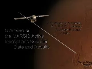
D. D. Morgan, D. A. Gurnett, R. L. Huff, D. L. Kirchner, A. J. Kopf, F. Jaeger, F. Duru. Overview of the MARSIS Active Ionospheric Sounder: Data and Results. Science Objectives. Characterize the response of the Martian ionosphere to various inputs:

E N D
D. D. Morgan, D. A. Gurnett, R. L. Huff, D. L. Kirchner, A. J. Kopf, F. Jaeger, F. Duru Overview of the MARSIS Active Ionospheric Sounder: Data and Results
Science Objectives Characterize the response of the Martian ionosphere to various inputs: • Solar EUV intensity • Energetic particles • Areodetic effects (seasons, latitude, local time) • Crustal magnetc fields • Solar wind
Targets of Opportunity • Spacecraft local electron density • Magnetic field • Absorption of surface reflection (indicator of energetic particles) • Multiple ionospheric reflection (indicator of plasma trapped in crustal magnetic field cusps) • Upper layers of ionosphere
Radar Reflections from the Ionosphere Gurnett et al. 2005, Science.
Mars Advanced Radar for Subsurface and Ionospheric Sounding (MARSIS) • Time resolution = 91.4 μs ~ ±6.8 km • Frequency resolution ≈10 kHz • 80 delay time bins to 7.5 ms • 160 frequency bins to 5.5 MHz
An Ionogram Duru et al., 2008, SWIM, San Diego
For electrons B=1/28Tc 1.25 ms 28.5 nT Akalin et al., 2008, SWIM, San Diego
MARSIS Active Ionospheric Sounder: Processing of Ionospheric Sounding Traces
Ionogram inversion • Time delay equation:
Inverting the delay time equation: lamination method (Jackson, 1969) • Assume fpe is monotonic function of range z • Assume horizontal stratification • Break into segments at instrument frequencies • Chose integrable functional form:
Inverting (continued) • Invert: • Change variables • Integrate
P-03-14 D. D. Morgan, D. A. Gurnett, D. L. Kirchner, J. L. Fox, E. Nielsen, J. J. Plaut, G. Picardi MARSIS Active Ionospheric Sounding Results
Procedure for using individual fits to Chapman model • Order samples by some parameter, e. g., , Time, F10.7, etc. • Place samples in bins of 100 • Take the average
1.57 AU < R < 1.67 AU 31 Jan. 2006 – 16 Feb. 2007 1.38 AU < R < 1.42 AU 16 Feb. 2007 – 31 Jul. 2007 1.39 AU < R < 1.48 AU 14 Aug. 2005 – 31 Jan. 2007
Conclusions (Morgan et al., 2008, accepted, J. Geophys. Res.) • d ln n0/d ln F10.7 = 0.31 ± 0.04, compared to Hantsch and Bauer (1990): 0.36 Fox and Yeager(2006): 0.29 – 0.41 for 60° ≤ χ ≤ 90° Breus et al. (2004): 0.37 • n0 varies between 1.4 to 1.8 x 105 cm-3, nearly constant with solar zenith angle and latitude • h0 varies between 110 and 140 km, falls off at χ > 60° due to oblique insolation but increases toward poles near summer solstice • H ~11 km for 0 < χ < 40°, increases to 15 km (270 K, 1.39 AU < R < 1.48 AU, late southern summer) 14 km (250 K, 1.57 AU < R < 1.67 AU, northern summer) 17 km (310 K, 1.38 AU < R < 1.42 AU, southern summer) • SEPs are associated with Δ n0/n0 of +6%, +Δ h0 of 3 km, ΔH of 7 km (??)
Morgan, D. D., D. A. Gurnett, D. L. Kirchner, J. L. Fox, E. Nielsen, and J. J. Plaut, Variation of the Martian ionospheric election density from Mars Express radar soundings, J. Geophys. Res., doi:10.1029/JA013313, accepted, 2008.
Investigation on the Magnetic Field Draping Near Mars from MARSIS F. Akalin1, D. A. Gurnett1, T. F. Averkamp1, D. L. Kirchner1, R. Modolo1, G. Chanteur2, M. H. Acuna3, J. E. P. Connerney3, J. R. Espley3, N. F. Ness4 1University of Iowa, Iowa City, IA 52240, USA 2CETP-IPSL, 10-12 Avenue de l’Europe, 78140 Velizy, France 3NASA Goddard Space Flight Center, Greenbelt, MD 20771, USA 4Inst. For Astrophysics and Computational Science, Catholic University of America, Washington, DC 20064, USA
OUTLINE • Electron cyclotron echoes and how they are produced. • Comparison of electron cyclotron echoes to Cain et al. model 1-Calculating the induced draped field vector 2-Determining MPB using electron number density and magnetic field • Statistics of all the magnetic field measurements without crustal field
For electrons B=1/28Tc 1.25 ms 28.5 nT
Bx=18.54±0.96 nT By=-16.22±0.58 nT Bz=-7.11±1.02 nT 1 Bx=11.59±0.91nT By=4.64±0.92 nT Bz=9.27±0.78 nT 2 1 2
Conclusion Limit of detectability of magnetic field by MARSIS, on dayside, coincides roughly with induced magnetosphere boundary.
Electron Densities and the Boundary Between the Ionosphere and the Solar Wind at Mars from Local Electron Plasma Oscillations F. Duru, D. A. Gurnett, D. D. Morgan, R. Modolo, A. F. Nagy, D. Najip and J. D. Winningham Chapman Conference on Solar Wind Interactions with Mars, Jan. 24, 2008, San Diego
Duru, F., D. A. Gurnett, D. D. Morgan, R. Modolo, A. F. Nagy, and D. Najib, Electron densities in the upper ionosphere of Mars from the excitation of electron plasma oscillations, J. Geophys. Res., accepted, 2008.
MARSIS on MEX(Mars Advanced Radar for Subsurface and Ionospheric Sounding) • Low-frequency radar sounder used for sounding of the ionosphere as well as subsurface sounding. • Consists of: An antenna subsystem, 40 m tip to tip dipole antenna, 7 m monopole antenna, a radio frequency subsystem, a digital electronic subsystem. • Radar soundings are performed by transmitting a short pulse of radio waves at a fixed frequency, and then measuring the time delay of the returning echo. • MARSIS also measures local electron density from the excitation of local electron plasma oscillations.
Local Electron Densities • As the transmitter steps in frequency strong local electrostatic oscillations, called Langmuir waves are excited, when f = fp. • The local electron plasma frequency can be used to obtain the electron density. ne = (fp/8980)2 cm-3, where fp is in Hz. • One of the advantages of this method is that the electron densities can be measured at very high altitudes, where remote soundings are not obtained. • This study is done at the altitudes between 275 km and 1300 km.
Electron Plasma Oscillation Harmonics • The excitation of electron plasma oscillations by the sounder transmitter creates harmonics of the local electron plasma frequency which are seen as closely spaced vertical lines in the upper left corner of the ionograms. • This is because, with voltage amplitudes on the antenna much greater than the power supply voltage in the preamplifier, the received waveforms are usually severely clipped. • In many cases, the fundamental of the electron plasma frequency cannot be observed, since it is below the lower limit of the frequency of the receiver. However, it can still be determined from the spacing of the harmonics which occur at higher frequencies.