Download
1 / 39
390 likes | 538 Vues
Mat-F February 21, 2005 Separation of variables. Åke Nordlund Niels Obers, Sigfus Johnsen / Anders Svensson Kristoffer Hauskov Andersen Peter Browne Rønne. Overview. Follow-up Computer problems Maple TA problems Maple TA changes New web pages Chapter 19 Separation of variables

E N D
Mat-FFebruary 21, 2005Separation of variables Åke Nordlund Niels Obers, Sigfus Johnsen / Anders Svensson Kristoffer Hauskov Andersen Peter Browne Rønne
Overview • Follow-up • Computer problems • Maple TA problems • Maple TA changes • New web pages • Chapter 19 • Separation of variables • Exercises today
Follow-up:Computer problems • Client-server problems • Over-loaded servers • Over-loaded network?? • Browser problems • Mozilla / Maple / JAVA • Netscape plugin missing • Don’t panic! • “… it said in warm, red letters …”
Follow-up:Computer problems • Some problems will be fixed • Browser: Netscape with plugin • Some hardware constraints need work-arounds • Network limitations?? • Possibly use D315 & A122 • CPU limitations • Make sure logins and windows are on localhost
Follow-up:Maple TA • Maple TA improvements • No longer accepts “0” or “whatever” as solutions • Remaining limitations • Still accepts less than general PDE solutions • Use human judgment! • I will !
Follow-up:Maple TA • Maple TA changes • For those who could not come Wednesday • For continued exercises (computer problems) • For additional training Maple TA exercises will be (are) available in an open version from the day (Thursday) after the exercises.
New web pages • Maple Examples • Examples / templates for turn-in assignments • Exercise Groups • Time & room schedule added • Rooms could possibly change next week • But not this week!
19. Partial Differential Equations:Separation of variables … • Main principles • Why? • Techniques • How?
Main principles • Why? • Because many systems in physics are separable • In particular systems with symmetries • Such as spherically symmetric problems Example: Spherical harmonics u(r,Θ,φ,t) = Ylmn(r,Θ,φ) eiωt
19. Partial Differential Equations:Separation of Variables … • Main principles • Why? • Common in physics! • Greatly simplifies things! • Techniques • How?
19.1 Separation of variables:the general method • Suppose we seek a PDE solution u(x,y,z,t) Ansatz: u(x,y,z,t) = X(x) Y(y) Z(z) T(t) This ansatz may be correct or incorrect! If correct we have u/x = X’(x) Y(y) Z(z) T(t) 2u/x2 = X”(x) Y(y) Z(z) T(t)
19.1 Separation of variables:the general method • Suppose we seek a PDE solution u(x,y,z,t): Ansatz: u(x,y,z,t) = X(x) Y(y) Z(z) T(t) This ansatz may be correct or incorrect! If correct we have u/y = X(x) Y’(y) Z(z) T(t) 2u/y2 = X(x) Y”(y) Z(z) T(t) u/y = X(x) Y’(y) Z(z) T(t) 2u/y2 = X(x) Y”(y) Z(z) T(t)
19.1 Separation of variables:the general method • Suppose we seek a PDE solution u(x,y,z,t): Ansatz: u(x,y,z,t) = X(x) Y(y) Z(z) T(t) This ansatz may be correct or incorrect! If correct we have u/y = X(x) Y’(y) Z(z) T(t) 2u/y2 = X(x) Y”(y) Z(z) T(t) u/z = X(x) Y(y) Z’(z) T(t) 2u/z2 = X(x) Y(y) Z”(z) T(t)
19.1 Separation of variables:the general method • Suppose we seek a PDE solution u(x,y,z,t): Ansatz: u(x,y,z,t) = X(x) Y(y) Z(z) T(t) This ansatz may be correct or incorrect! If correct we have u/y = X(x) Y’(y) Z(z) T(t) 2u/y2 = X(x) Y”(y) Z(z) T(t) u/t = X(x) Y(y) Z(z) T’(t) 2u/t2 = X(x) Y(y) Z(z) T”(t)
Examples u(x,y,z,t) = xyz2sin(bt) u(x,y,z,t) = xy + zt u(x,y,z,t) = (x2+y2) z cos(ωt)
Yes! No! ? Hm… Examples Separable? u(x,y,z,t) = xyz2sin(bt) u(x,y,z,t) = xy + zt u(x,y,z,t) = (x2+y2) z cos(ωt)
Yes! No! ? Hm… (x2+y2) p2 Examples Separable? u(x,y,z,t) = xyz2sin(bt) u(x,y,z,t) = xy + zt u(x,y,z,t) = (x2+y2) z cos(ωt)
Yes! Yes! No! Examples Separable? u(x,y,z,t) = xyz2sin(bt) u(x,y,z,t) = xy + zt u(p,z,t) = p2 z cos(ωt)
Example PDEs • The wave equation where c22u= 2u/t2 2 2/x2 + 2/y2 + 2/z2 Ansatz: u(x,y,z,t) = X(x) Y(y) Z(z) T(t)
Separation of variables in the wave equation • For the ansatz to work we must have (lets set c=1 for now to get rid of a triviality!) • Divide though with XYZT, for: X”YZT + XY”ZT + XYZ”T = XYZT” X”/X + Y”/Y + Z”/Z = T”/T This can only work if all of these are constants!
Separation of variables in the wave equation • Let’s take all the constants to be negative • Negative bounded behavior at large x,y,z,t X”/X + Y”/Y + Z”/Z = T”/T These are called separation constants - 2 - 2 - 2 = - µ2 This is typical: If / when a PDE allows separation of variables, the partial derivatives are replaced with ordinary derivatives, and all that remains of the PDE is an algebraic equation and a set of ODEs – much easier to solve!
Separation of variables in the wave equation • Solutions of the ODEs: Example: x-direction X”/X = - 2 General solution: X(x) = A exp(i x) + B exp(-i x) or X(x) = A’ cos( x) + B’ sin( x)
Separation of variables in the wave equation • Combining all directions (and time) Example: u = exp(i x) exp(i y) exp(i x) exp(-i cµt) or u = exp(i ( x + y + x -ω t)) This is a traveling wave, with wave vector {,,} and frequencyω. A general solution of the wave equation is a super-position of such waves.
Example PDEs • The diffusion equation where 2u= u/t 2 2/x2 + 2/y2 + 2/z2 Ansatz: u(x,y,z,t) = X(x) Y(y) Z(z) T(t)
Separation of variables in the diffusion equation • For the ansatz to work we must have (lets set =1 for now to again get rid of that triviality) • Divide though with XYZT, for: X”YZT + XY”ZT + XYZ”T = XYZT’ X”/X + Y”/Y + Z”/Z = T’/T Again, this can only work if all of these are constants!
Separation of variables in the diffusion equation • Again, we take all the constants to be negative • Negative bounded behavior at large x,y,z,t X”/X + Y”/Y + Z”/Z = T’/T - 2 - 2 - 2 = - µ We see the typical behavior again: All that remains of the PDE is an algebraic equation and a set of ODEs – much easier to solve!
Separation of variables in the diffusion equation • Solutions of the ODEs: Example: x-direction X”/X = - 2 General solution: X(x) = A exp(i x) + B exp(-i x) or X(x) = A’ cos( x) + B’ sin( x)
Separation of variables in the diffusion equation Time-direction: T’/T = - µ General solution: T(t) = A exp(-µ t) + B exp(µ t)
Separation of variables in the diffusion equation • Combining all directions (and time) Example: u = exp(i x) exp(i y) exp(i x) exp(-µ t) or u = exp(i ( x + y + x )) exp(-µ t) This is a damped wave, with wave vector {,,} and damping constantµ. A general solution of the diffusion equation is a super-position of such waves.
Example PDEs • The Laplace equation where 2u= 0 2 2/x2 + 2/y2 + 2/z2 Ansatz: u(x,y,z,t) = X(x) Y(y) Z(z)
Separation of variables in the Laplace equation • For the ansatz to work we must have • Divide though with XYZT, for: X”YZT + XY”ZT + XYZ”T = 0 X”/X + Y”/Y + Z”/Z = 0 Again, this can only work if all of these are constants!
Separation of variables in the Laplace equation • This time we cannot take all constants to be negative! Let’s assume for simplicity (as in the example in the book) that there is only x & y dependence! X”/X + Y”/Y + Z”/Z = 0 - 2 - 2 - 2 = 0 At least one of the terms must be positive imaginary wave number; i.e., exponential rather than sinusoidal behavior!
Separation of variables in the Laplace equation • Solutions of the ODEs: Example: x-direction X”/X = - 2 < 0 assumed General solution: X(x) = A exp(i x) + B exp(-i x) or X(x) = A’ cos( x) + B’ sin( x)
Separation of variables in the Laplace equation • Solutions of the ODEs: Example: y-direction Y”/Y = + 2 > 0 follows! General solution: Y(y) = C exp( y) + D exp(- y) or Y(y) = C’ cosh( y) + B’ sinh( y)
Separation of variables in the Laplace equation • Combining x & y directions Example: u= [A exp(i x) + B exp(-i x)] [C exp( y) + D exp(- y)] or u= [A’ cos( x) + B’ sin( x)] [C’ cosh( y) + D’ sinh(- y)] A general solution of the Laplace equation is a superposition of such functions (which everywhere have a ’saddle-like’ behavior – net curvature = 0)
19.2 Superposition of separated solutions • If the PDE with separable solutions is linear … • Wave equation • Diffusion equation • Laplace & Poisson eq. • Schrødinger eq. • … then any linear combination (superposition) is also a solution • Boundary conditions will make a limited selection!
Exercises today: • Exercise 19.1 • Separation of variables • Exercise 19.2 • Diffusion of heat • Exercise 19.3 • Wave equation on a stretched membrane
Examples in the text of the book 2u= u/t • Heat diffusion • Stationary (u/t = 0) • equivalent to Laplace equation problem! • Various boundary conditions • selects particular solutions • NOTE: a diffusion (heat flow) equation may well have a mixed sinusoidal & exponential behavior in space! • consider the limit when the time dependence is weak! 2u= 0 - 2 - 2 - 2 = - µ→ 0 2u= (1/)u/t → 0
Enough for today! Good luck with the exercises 10:15-12:00