Download
1 / 64
650 likes | 672 Vues
Explore the impact, benefits, and challenges of multicores from a compiler's viewpoint, examining issues such as power, efficiency, complexity, and communication bandwidth. Learn about the transition from multiprocessors to multicores and the criteria for compiler success in handling diverse programs and environments.

E N D
Multicores from the Compiler's Perspective A Blessing or A Curse? Saman Amarasinghe Associate Professor, Massachusetts Institute of Technology Department of Electrical Engineering and Computer Science Computer Science and Artificial Intelligence Laboratory CTO, Determina Inc.
IBM Power 6Dual Core IBM Power 4 and 5Dual Cores Since 2001 … 2H 2004 1H 2005 2H 2005 1H 2006 2H 2006 Multicores are coming! MIT Raw 16 CoresSince 2002 Intel Montecito1.7 Billion transistorsDual Core IA/64 Intel TanglewoodDual Core IA/64 Intel Pentium D (Smithfield) Intel Dempsey Dual Core Xeon Intel Pentium Extreme3.2GHz Dual Core Cancelled Intel Tejas & JayhawkUnicore (4GHz P4) Intel YonahDual Core Mobile AMD OpteronDual Core Sun Olympus and Niagara8 Processor Cores IBM CellScalable Multicore
What is Multicore? • Multiple, externally visible processors on a single die where the processors have independent control-flow, separate internal state and no critical resource sharing. • Multicores have many names… • Chip Multiprocessor (CMP) • Tiled Processor • ….
Why move to Multicores? • Many issues with scaling a unicore • Power • Efficiency • Complexity • Wire Delay • Diminishing returns from optimizing a single instruction stream
Itanium 2 (421mm2 / .18) Floating Point Integer Core Pentium 4 (217mm2 / .18) Decode Fetch Bus Control Trace Cache L2 Data Cache FPUMMX/SSE Integer Core Renaming L2 Data Cache Op Scheduling 4004 (12mm2 / 8) Moore’s Law: Transistors Well Spent? transistors 1,000,000,000 Itanium 2 Itanium 100,000,000 P4 P3 10,000,000 P2 Pentium 486 1,000,000 386 286 100,000 8086 10,000 8080 8008 Moore’s Law 4004 1,000 1970 1975 1980 1985 1990 1995 2000 2005
Outline • Introduction • Overview of Multicores • Success Criteria for a Compiler • Data Level Parallelism • Instruction Level Parallelism • Language Exposed Parallelism • Conclusion
Impact of Multicores • How does going from Multiprocessors to Multicores impact programs? • What changed? • Where is the Impact? • Communication Bandwidth • Communication Latency
Communication Bandwidth • How much data can be communicated between two cores? • What changed? • Number of Wires • IO is the true bottleneck • On-chip wire density is very high • Clock rate • IO is slower than on-chip • Multiplexing • No sharing of pins • Impact on programming model? • Massive data exchange is possible • Data movement is not the bottleneck locality is not that important 10,000X 32 Giga bits/sec ~300 Tera bits/sec
Communication Latency • How long does it take for a round trip communication? • What changed? • Length of wire • Very short wires are faster • Pipeline stages • No multiplexing • On-chip is much closer • Impact on programming model? • Ultra-fast synchronization • Can run real-time apps on multiple cores 50X ~200 Cycles ~4 cycles
PE PE $$ X $$ X PE PE $$ X $$ X Memory Memory Past, Present and the Future? Traditional Multiprocessor Basic Multicore IBM Power5 Integrated Multicore 16 Tile MIT Raw PE PE PE PE $$ $$ $$ $$ Memory Memory Memory Memory
Outline • Introduction • Overview of Multicores • Success Criteria for a Compiler • Data Level Parallelism • Instruction Level Parallelism • Language Exposed Parallelism • Conclusion
When is a compiler successful as a general purpose tool? • General Purpose • Programs compiled with the compiler are in daily use by non-expert users • Used by many programmers • Used in open source and commercial settings • Research / niche • You know the names of all the users
Success Criteria • Effective • Stable • General • Scalable • Simple
1: Effective • Good performance improvements on most programs • The speedup graph goes here!
2: Stable • Simple change in the program should not drastically change the performance! • Otherwise need to understand the compiler inside-out • Programmers want to treat the compiler as a black box
3: General • Support the diversity of programs • Support Real Languages: C, C++, (Java) • Handle rich control and data structures • Tolerate aliasing of pointers • Support Real Environments • Separate compilation • Statically and dynamically linked libraries • Work beyond an ideal laboratory setting
4: Scalable • Real applications are large! • Algorithm should scale • polynomial or exponential in the program size doesn’t work • Real Programs are Dynamic • Dynamically loaded libraries • Dynamically generated code • Whole program analysis tractable?
5: Simple • Aggressive analysis and complex transformation lead to: • Buggy compilers! • Programmers want to trust their compiler! • How do you manage a software project when the compiler is broken? • Long time to develop • Simple compiler fast compile-times • Current compilers are too complex!
Outline • Introduction • Overview of Multicores • Success Criteriafor a Compiler • Data Level Parallelism • Instruction Level Parallelism • Language Exposed Parallelism • Conclusion
Identify loops where each iteration can run in parallel DOALL parallelism What affects performance? Parallelism Coverage Granularity of Parallelism Data Locality TDT = DT MP1 = M+1 NP1 = N+1 EL = N*DX PI = 4.D0*ATAN(1.D0) TPI = PI+PI DI = TPI/M DJ = TPI/N PCF = PI*PI*A*A/(EL*EL) DO 50 J=1,NP1 DO 50 I=1,MP1 PSI(I,J) = A*SIN(( I-.5D0)*DI)* SIN((J-.5D0)*DJ) P(I,J) = PCF*(COS(2.D0) CONTINUE DO 60 J=1,N DO 60 I=1,M U(I+1,J) = -(PSI(I+1,J+1) -PSI(I+1,J))/DY V(I,J+1) = (PSI(I+1,J+1)- PSI(I,J+1))/DX CONTINUE Data Level Parallelism TIME processors
Amdahl’s Law Performance improvement to be gained from faster mode of execution is limited by the fraction of the time the faster mode can be used Find more parallelism Interprocedural analysis Alias analysis Data-flow analysis …… Parallelism Coverage More processors processors
SUIF Parallelizer Results Parallelism Coverage S p e e d u p SPEC95fp, SPEC92fp, Nas, Perfect Benchmark Suites On a 8 processor Silicon Graphics Challenge (200MHz MIPS R4000)
Synchronization is expensive Need to find very large parallel regions coarse-grain loop nests Heroic analysis required TDT = DT MP1 = M+1 NP1 = N+1 EL = N*DX PI = 4.D0*ATAN(1.D0) TPI = PI+PI DI = TPI/M DJ = TPI/N PCF = PI*PI*A*A/(EL*EL) DO 50 J=1,NP1 DO 50 I=1,MP1 PSI(I,J) = A*SIN(( I-.5D0)*DI)* SIN((J-.5D0)*DJ) P(I,J) = PCF*(COS(2.D0) CONTINUE DO 60 J=1,N DO 60 I=1,M U(I+1,J) = -(PSI(I+1,J+1) -PSI(I+1,J))/DY V(I,J+1) = (PSI(I+1,J+1)- PSI(I,J+1))/DX CONTINUE Granularity of Parallelism TIME processors
Granularity of Parallelism • Synchronization is expensive • Need to find very large parallel regions coarse-grain loop nests • Heroic analysis required • Single unanalyzable line turb3d in SPEC95fp
Granularity of Parallelism • Synchronization is expensive • Need to find very large parallel regions coarse-grain loop nests • Heroic analysis required • Single unanalyzable line • Small Reduction in Coverage • Drastic Reduction in Granularity turb3d in SPEC95fp
SUIF Parallelizer Results Parallelism Coverage S p e e d u p Granularity of Parallelism
SUIF Parallelizer Results Parallelism Coverage S p e e d u p Granularity of Parallelism
Data Locality • Non-local data • Stalls due to latency • Serialize when lack of bandwidth • Data Transformations • Global impact • Whole program analysis A[0] A[1] A[2] A[3] A[4] A[5] A[6] A[7] A[8] A[9] A[10] A[11] A[12] A[13] A[14] A[15]
DLP on Multiprocessors:Current State • Huge body of work over the years. • Vectorization in the ’80s • High Performance Computing in ’90s • Commercial DLP compilers exist • But…only a very small user community • Can multicores make DLP mainstream? ?
Effectiveness • Main Issue • Parallelism Coverage • Compiling to Multiprocessors • Amdahl’s law • Many programs have no loop-level parallelism • Compiling to Multicores • Nothing much has changed
Main Issue Granularity of Parallelism Compiling for Multiprocessors Unpredictable, drastic granularity changes reduce the stability Compiling for Multicores Low latency granularity is less important Stability
Main Issue Changes in general purpose programming styles over time impacts compilation Compiling for Multiprocessors (In the good old days) Mainly FORTRAN Loop nests and Arrays Compiling for Multicores Modern languages/programs are hard to analyze Aliasing (C, C++ and Java) Complex structures (lists, sets, trees) Complex control (concurrency, recursion) Dynamic (DLLs, Dynamically generated code) Generality
Main Issue Whole program analysis and global transformations don’t scale Compiling for Multiprocessors Interprocedural analysis needed to improve granularity Most data transformations have global impact Compiling for Multicores High bandwidth and low latency no data transformations Low latency granularity improvements not important Scalability
Main Issue Parallelizing compilers are exceedingly complex Compiling for Multiprocessors Heroic interprocedural analysis and global transformations are required because of high latency and low bandwidth Compiling for Multicores Hardware is a lot more forgiving… But…modern languages and programs make life difficult Simplicity
Outline • Introduction • Overview of Multicores • Success Criteria for a Compiler • Data Level Parallelism • Instruction Level Parallelism • Language Exposed Parallelism • Conclusion
seed.0=seed pval1=seed.0*3.0 v1.2=v1 v2.4=v2 pval5=seed.0*6.0 pval2=seed.0*v1.2 pval0=pval1+2.0 pval3=seed.o*v2.4 pval4=pval5+2.0 tmp1.3=pval2+2.0 tmp0.1=pval0/2.0 tmp2.5=pval3+2.0 tmp3.6=pval4/3.0 tmp1=tmp1.3 tmp0=tmp0.1 tmp2=tmp2.5 pval7=tmp1.3+tmp2.5 tmp3=tmp3.6 pval6=tmp1.3-tmp2.5 v1.8=pval7*3.0 v2.7=pval6*5.0 v0.9=tmp0.1-v1.8 v1=v1.8 v3.10=tmp3.6-v2.7 v0=v0.9 v2=v2.7 v3=v3.10 Instruction Level parallelism on a Unicore • Programs have ILP • Modern processors extract the ILP • Superscalars Hardware • VLIW Compiler tmp0 = (seed*3+2)/2 tmp1 = seed*v1+2 tmp2 = seed*v2 + 2 tmp3 = (seed*6+2)/3 v2 = (tmp1 - tmp3)*5 v1 = (tmp1 + tmp2)*3 v0 = tmp0 - v1 v3 = tmp3 - v2
ALU ALU ALU ALU ALU ALU ALU ALU ALU ALU ALU ALU ALU ALU ALU ALU Register File Bypass Network Scalar Operand Network (SON) • Moves results of an operation to dependent instructions • Superscalars in Hardware • What makes a good SON? seed.0=seed pval5=seed.0*6.0
Scalar Operand Network (SON) • Moves results of an operation to dependent instructions • Superscalars in Hardware • What makes a good SON? • Low latency from producer to consumer seed.0=seed pval5=seed.0*6.0 seed.0=seed pval5=seed.0*6.0
Scalar Operand Network (SON) • Moves results of an operation to dependent instructions • Superscalars in Hardware • What makes a good SON? • Low latency from producer to consumer • Low occupancy at the producer and consumer seed.0=seed pval5=seed.0*6.0 seed.0=seed lock Write mem unlock Test lock Branch Test lock Branch Test lock Branch Test lock Branch Read memory pval5=seed.0*6.0
Scalar Operand Network (SON) • Moves results of an operation to dependent instructions • Superscalars in Hardware • What makes a good SON? • Low latency from producer to consumer • Low occupancy at the producer and consumer • High bandwidth for multiple operations v1.2=v1 seed.0=seed v2.4=v2 pval2=seed.0*v1.2 pval5=seed.0*6.0 pval3=seed.o*v2.4 tmp2.5=pval3+2.0 tmp1.3=pval2+2.0 pval7=tmp1.3+tmp2.5 tmp1=tmp1.3 seed.0=seed pval5=seed.0*6.0
Is an Integrated Multcore Reedy to be a Scalar Operand Network? Traditional Multiprocessor Basic Multicore Integrated Multicore VLIW Unicore
Scalable Scalar Operand Network? Integrated Multicore Unicore • Unicores • N2 connectivity • Need to cluster introduces latency • Integrated Multicores • No bottlenecks in scaling
seed.0=seed pval1=seed.0*3.0 v1.2=v1 v2.4=v2 pval5=seed.0*6.0 pval2=seed.0*v1.2 pval0=pval1+2.0 pval3=seed.o*v2.4 pval4=pval5+2.0 tmp1.3=pval2+2.0 tmp0.1=pval0/2.0 tmp2.5=pval3+2.0 tmp3.6=pval4/3.0 tmp1=tmp1.3 tmp0=tmp0.1 tmp2=tmp2.5 pval7=tmp1.3+tmp2.5 tmp3=tmp3.6 pval6=tmp1.3-tmp2.5 v1.8=pval7*3.0 v2.7=pval6*5.0 v0.9=tmp0.1-v1.8 v1=v1.8 v3.10=tmp3.6-v2.7 v0=v0.9 v2=v2.7 v3=v3.10 Compiler Support for Instruction Level Parallelism • Accepted general purpose technique • Enhance the performance of superscalars • Essential for VLIW • Instruction Scheduling • List scheduling or Software pipelining seed.0=recv() seed.0=recv() pval5=seed.0*6.0 pval2=seed.0*v1.2 pval4=pval5+2.0 tmp1.3=pval2+2.0 tmp3.6=pval4/3.0 send(tmp1.3) tmp3=tmp3.6 tmp1=tmp1.3 v2.7=recv() tmp2.5=recv() v3.10=tmp3.6-v2.7 pval7=tmp1.3+tmp2.5 v3=v3.10 v1.8=pval7*3.0 v1=v1.8 tmp0.1=recv() v1=v1.8 v0.9=tmp0.1-v1.8 tmp0.1=recv() v0.9=tmp0.1-v1.8 v0=v0.9 v0=v0.9
seed.0=seed v1.2=v1 seed.0=seed v2.4=v2 send(seed.0) pval1=seed.0*3.0 route(t,E) route(t,E) route(N,t) route(W,t) seed.0=recv(0) seed.0=recv() route(W,S) pval3=seed.o*v2.4 pval5=seed.0*6.0 route(N,t) seed.0=recv() pval0=pval1+2.0 pval2=seed.0*v1.2 tmp0.1=pval0/2.0 pval1=seed.0*3.0 v1.2=v1 pval4=pval5+2.0 tmp2.5=pval3+2.0 v2.4=v2 tmp3.6=pval4/3.0 tmp1.3=pval2+2.0 tmp2=tmp2.5 pval5=seed.0*6.0 send(tmp2.5) send(tmp1.3) route(t,E) pval2=seed.0*v1.2 pval0=pval1+2.0 send(tmp0.1) route(t,W) tmp3=tmp3.6 tmp1=tmp1.3 tmp0=tmp0.1 route(E,t) route(t,E) pval3=seed.o*v2.4 tmp1.3=recv() route(W,t) route(W,S) pval4=pval5+2.0 tmp2.5=recv() pval6=tmp1.3-tmp2.5 route(W,S) tmp1.3=pval2+2.0 pval7=tmp1.3+tmp2.5 route(N,t) v2.7=pval6*5.0 tmp0.1=pval0/2.0 v1.8=pval7*3.0 tmp2.5=pval3+2.0 seed.0=seed tmp3.6=pval4/3.0 tmp1=tmp1.3 Send(v2.7) v1=v1.8 v2=v2.7 route(t,E) tmp0.1=recv() route(W,N) tmp0=tmp0.1 tmp2=tmp2.5 v0.9=tmp0.1-v1.8 route(W,N) pval1=seed.0*3.0 v1.2=v1 pval7=tmp1.3+tmp2.5 tmp3=tmp3.6 route(S,t) v2.4=v2 v0=v0.9 v2.7=recv() pval5=seed.0*6.0 v3.10=tmp3.6-v2.7 pval2=seed.0*v1.2 pval6=tmp1.3-tmp2.5 pval0=pval1+2.0 pval3=seed.o*v2.4 v3=v3.10 pval4=pval5+2.0 tmp1.3=pval2+2.0 v1.8=pval7*3.0 tmp0.1=pval0/2.0 tmp2.5=pval3+2.0 tmp3.6=pval4/3.0 v2.7=pval6*5.0 tmp1=tmp1.3 tmp0=tmp0.1 tmp2=tmp2.5 v0.9=tmp0.1-v1.8 pval7=tmp1.3+tmp2.5 tmp3=tmp3.6 pval6=tmp1.3-tmp2.5 v1=v1.8 v3.10=tmp3.6-v2.7 v1.8=pval7*3.0 v2.7=pval6*5.0 v0=v0.9 v2=v2.7 v0.9=tmp0.1-v1.8 v3=v3.10 v1=v1.8 v3.10=tmp3.6-v2.7 v0=v0.9 v2=v2.7 v3=v3.10 ILP on Integrated Multicores:Space-Time Instruction Scheduling • Partition, placement, route and schedule • Similar to Clustered VLIW
x = cmp a, b • • • • • • br x • • • • • • br x • • • br x • • • • • • br x Handling Control Flow • Asynchronous global branching • Propagate the branch condition to all the tiles as part of the basic block schedule • When finished with the basic block execution asynchronously switch to another basic block schedule depending on the branch condition
Raw Performance Dense Matrix Multimedia Irregular • 32 tile Raw
Success Criteria integrated multicore • Effective • If ILP exists same • Stable • Localized optimization similar • General • Applies to same type of applications • Scalable • Local analysis similar • Simple • Deeper analysis and more transformations unicore
Outline • Introduction • Overview of Multicores • Success Criteria for a Compiler • Data Level Parallelism • Instruction Level Parallelism • Language Exposed Parallelism • Conclusion
C von-Neumannmachine Languages are out-of-touch with Architecture Modern architecture • Two choices: • Develop cool architecture with complicated, ad-hoc language • Bend over backwards to supportold languages like C/C++
Supporting von Neumann Languages • Why C (FORTRAN, C++ etc.) became very successful? • Abstracted out the differences of von Neumann machines • Register set structure • Functional units and capabilities • Pipeline depth/width • Memory/cache organization • Directly expose the common properties • Single memory image • Single control-flow • A clear notion of time • Can have a very efficient mapping to a von Neumann machine • “C is the portable machine language for von Numann machines” • Today von Neumann languages are a curse • We have squeezed out all the performance out of C • We can build more powerful machines • But, cannot map C into next generation machines • Need better languages with more information for optimization