Understanding Production Possibilities: Opportunity Cost and Economic Efficiency
This chapter explores fundamental concepts in economics, focusing on the production possibilities frontier (PPF) and opportunity cost. It defines the PPF, illustrates efficient resource allocation, and examines the impact of specialization and trade on production capabilities. Readers will learn how to calculate opportunity costs and understand the implications of trade-offs in production decisions. The chapter emphasizes the relationship between current production choices and future possibilities, providing a comprehensive overview of economic efficiency and the role of marginal costs and benefits in decision-making.

Understanding Production Possibilities: Opportunity Cost and Economic Efficiency
E N D
Presentation Transcript
2 CHAPTER The Economic Problem
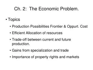
After studying this chapter you will be able to • Define the production possibilities frontier and calculate opportunity cost • Distinguish between production possibilities and preferences and describe an efficient allocation of resources • Explain how current production choices expand future production possibilities • Explain how specialization and trade expand our production possibilities • Describe the economic institutions that coordinate decisions
Production Possibilities and Opportunity Cost • The production possibilities frontier (PPF) is the boundary between those combinations of goods and services that can be produced and those that cannot. • To illustrate the PPF, we focus on two goods at a time and hold the quantities of all other goods and services constant. • That is, we look at a model economy in which everything remains the same (ceteris paribus) except the two goods we’re considering.
Production Possibilities and Opportunity Cost • Production Possibilities Frontier • Figure 2.1 shows the PPF for two goods: CDs and pizza. • Any point on the frontier such as E and any point inside the PPF such as Z are attainable. • Points outside the PPF are unattainable.
Production Possibilities and Opportunity Cost • Production Efficiency • We achieve production efficiency if we cannot produce more of one good without producing less of some other good. • Points on the frontier are efficient.
Production Possibilities and Opportunity Cost • Any point inside the frontier, such as Z, is inefficient. • At such a point, it is possible to produce more of one good without producing less of the other good. • At Z, resources are either unemployed or misallocated.
Production Possibilities and Opportunity Cost • Tradeoff Along the PPF • Every choice along the PPF involves a tradeoff. • On this PPF, we must give up some CDs to get more pizzas or give up some pizzas to get more CDs.
Production Possibilities and Opportunity Cost • Opportunity Cost • The PPF makes the concept of opportunity cost precise. • As we move down along the PPF, we produce more pizzas but the quantity of CDs we can produce decreases. • The opportunity cost of a pizza is the CDs forgone.
Production Possibilities and Opportunity Cost • In moving from E to F, the quantity of pizzas produced increases by 1 million. • The quantity of CDs produced decreases by 5 million. • The opportunity cost of producing the fifth 1 million pizzas is 5 million CDs. • One of these pizzas costs 5 CDs.
Production Possibilities and Opportunity Cost • In moving from F to E, the quantity of CDs produced increases by 5 million. • The quantity of pizzas produced decreases by 1 million. • The opportunity cost of the first 5 million CDs is 1 million pizzas. • One of these CDs costs 1/5 of a pizza.
Production Possibilities and Opportunity Cost • Note that the opportunity cost of a CD is the inverse of the opportunity cost of a pizza. • One pizza costs 5 CDs. • One CD costs 1/5 of a pizza.
Production Possibilities and Opportunity Cost • Because resources are not all equally productive in all activities, the PPF bows outward—is concave. • The outward bow of the PPF means that as the quantity produced of each good increases, so does its opportunity cost.
Using Resources Efficiently • All the points along the PPF are efficient. • To determine which of the alternative efficient quantities to produce, we compare costs and benefits. • The PPF and Marginal Cost • The PPF determines opportunity cost. • The marginal cost of a good or service is the opportunity cost of producing one more unit of it.
Using Resources Efficiently • Figure 2.2 illustrates the marginal cost of pizza. • As we move along the PPF in part (a), the opportunity cost of pizza increases. • The opportunity cost of producing one more pizza is the marginal cost of a pizza.
Using Resources Efficiently • In part (b) of Fig. 2.2, the bars illustrate the increasing opportunity cost of pizza. • The black dots • and the line labeled MC show the marginal cost of pizza. • The MC curve passes through the center of each bar.
Using Resources Efficiently • Preferences and Marginal Benefit • Preferences are a description of a person’s likes and dislikes. • To describe preferences, economists use the concepts of marginal benefit and the marginal benefit curve. • The marginal benefit of a good or service is the benefit received from consuming one more unit of it. • We measure marginal benefit by the amount that a person is willing to pay for an additional unit of a good or service.
Using Resources Efficiently • It is a general principle that the more we have of any good, the smaller is its marginal benefit and the less we are willing to pay for an additional unit of it. • We call this general principle the principle of decreasing marginal benefit. • The marginal benefit curve shows the relationship between the marginal benefit of a good and the quantity of that good consumed.
Using Resources Efficiently • Figure 2.3 shows a marginal benefit curve. • The curve slopes downward to reflect the principle of decreasing marginal benefit. • At point A, with pizza production at 0.5 million, people are willing to pay 5 CDs for a pizza.
Using Resources Efficiently • At point B, with pizza production at 1.5 million, people are willing to pay 4 CDs for a pizza. • At point E, with pizza production at 4.5 million, people are willing to pay 1 CD for a pizza.
Using Resources Efficiently • Efficient Use of Resources • When we cannot produce more of any one good without giving up some other good, we have achieved production efficiency. • We are producing at a point on the PPF. • When we cannot produce more of any one good without giving up some other good that we value more highly, we have achieved allocative efficiency. • We are producing at the point on the PPF that we prefer above all other points.
Using Resources Efficiently • Figure 2.4 illustrates allocative efficiency. • The point of allocative efficiency is the point on the PPF at which marginal benefit equals marginal cost. • This point is determined by the quantity at which the marginal benefit curve intersects the marginal cost curve.
Using Resources Efficiently • If we produce fewer than 2.5 million pizzas, marginal benefit exceeds marginal cost. • We get more value from our resources by producing more pizzas. • On the PPF at point A, we are producing too many CDs, and we are better off moving along the PPF to produce more pizzas.
Using Resources Efficiently • If we produce more than 2.5 million pizzas, marginal cost exceeds marginal benefit. • We get more value from our resources by producing fewer pizzas. • On the PPF at point C, we are producing too many pizzas, and we are better off moving along the PPF to produce fewer pizzas.
Using Resources Efficiently • If we produce exactly 2.5 million pizzas, marginal cost equals marginal benefit. • We cannot get more value from our resources. • On the PPF at point B, we are producing the efficient quantities of CDs and pizzas.
Economic Growth • The expansion of production possibilities—and increase in the standard of living—is called economic growth. • Two key factors influence economic growth: • Technological change • Capital accumulation • Technological change is the development of new goods and of better ways of producing goods and services. • Capital accumulation is the growth of capital resources, which includes human capital.
Economic Growth • The Cost of Economic Growth • To use resources in research and development and to produce new capital, we must decrease our production of consumption goods and services. • So economic growth is not free. • The opportunity cost of economic growth is less current consumption.
Economic Growth • Economic Growth in the United States and Hong Kong • In 1966, Hong Kong’s production possibilities (per person) were a quarter of those in the United States.
Economic Growth • By 2006, Hong Kong’s production possibilities (per person) were 80 percent of those in the United States. • Hong Kong’s PPF shifted out more quickly than did the U.S. PPF because Hong Kong devoted more of its resources to capital accumulation.
Economic Coordination • To reap the gains from trade, the choices of individuals must be coordinated. • To make coordination work, four complimentary social institutions have evolved over the centuries: • Firms • Markets • Property rights • Money
Economic Coordination • A firm is an economic unit that hires factors of production and organizes those factors to produce and sell goods and services. • A market is any arrangement that enables buyers and sellers to get information and do business with each other. • Property rights are the social arrangements that govern ownership, use, and disposal of resources, goods or services. • Money is any commodity or token that is generally acceptable as a means of payment.
Economic Coordination • Circular Flows Through Markets • A circular flow diagram, like Figure 2.8 on the next slide, illustrates how households and firms interact in the market economy.
Economic Coordination • Circular Flows Through Markets • Figure 2.8 illustrates how households and firms interact in the market economy. • Factors of production and goods and services flow in one direction. • And money flows in the opposite direction.
Economic Coordination • Coordinating Decisions • Markets coordinate individual decisions through price adjustments.