Understanding Surface Composition Distribution in Wright Valley, Antarctica

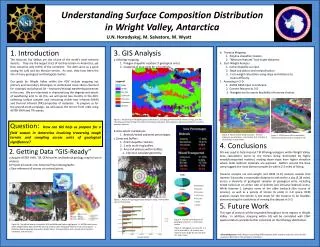
1. Understanding Surface Composition Distribution in Wright Valley, Antarctica U.N. Horodyskyj, M. Salvatore, M. Wyatt • Traverse Mapping • 1. Polyline shapefile creation. • 2. “Measure features” tool to get distances. • Cost-Weight Analysis • 1. Camp shapefile as input. • 2. Slope calculation and reclassification. • 3. Cost-weight calculation using slope and distance to • assess difficulty. • Assessing in 3-D • 1. ASTER DEM input to ArcScene. • 2. Convert features to 3-D. • 3. Navigate tool to assess feasibility of traverse choices. 3. GIS Analysis 1. Introduction The Antarctic Dry Valleys are site of one of the world’s most extreme deserts. They are the largest tract of ice-free terrain in Antarctica, yet they comprise only 0.03% of the continent. The ADV serve as a good analog for cold and dry Martian terrain. As such, they have been the site of many geological and biological studies. Our goals for Wright Valley within the ADV include mapping out primary and secondary lithologies to understand more about chemical (ie- coatings) and physical (ie – transport/mixing) weathering processes in the area. We are interested in characterizing the degrees and extent of weathering and, to do this, we will spend two months in the ADV, collecting surface samples and measuring visible-near infrared (VNIR) and thermal infrared (TIR) properties of materials. To prepare us for the ground-truth campaign, we will assess the terrain from orbit using ASTER VNIR and TIR scenes. • 3. GIS Analysis • Lithology mapping • 1. Polygon shapefile creation (7 geological units). • 2. Snapping of map units for smoothness. • Figure 2. ArcGIS map of TIR geological unit distribution, including primary bedrock units as in Fig.1, but also including secondary mixing units such as DI (dolerite-intrusive), SD (sandstone-dolerite) and Dol (SD + primary dolerite) mixtures. • Area extent calculations • 1. Bedrock/mixed sediment percentages. • Camp and Buffers • 1. Point shapefile creation. • 2. 1 mile multi-ring buffers. • 3. Area calculations within buffers. • a. Clip tool; calculate geometry. • Figure 3. Result of clipping geological polygons using 1-mile buffers • (out to three miles). Harder Question: How can GIS help us prepare for a field season in Antarctica involving traversing tough terrain and sampling across units of geological significance? Figure 6. Result of cost-weight analysis. Traverse distances are as follows; 1 (2.6 miles); 2 (5.77 miles); 3 (3.28 miles); 4 (2.88 miles). Figure 7. ASTER scene (30 m resolution), traverses and base camp as viewed in 3-D. 4. Conclusions GIS was used to help map out TIR lithology polygons within Wright Valley. Area calculations point to the terrain being dominated by highly mixed/transported material, eroding down-slope from higher elevation where older bedrock materials are exposed. Buffers around the base camp suggest the most diverse samples lie within 2-3 miles of hiking. Traverse analysis via cost-weight and DEM (3-D) analysis reveals that traverse 3 provides a reasonable distance to trek within a day (3.28 miles) across a diversity of geological samples (6 geological units, including mixed colluvium on either side of dolerite and intrusive bedrock units). While traverse 1 samples some of the older bedrock (the source of erosion), as well as a variety of terrain (6 units) in 2-D space, DEM analysis reveals the terrain is too steep for the traverse to be feasible, demonstrating the usefulness of viewing this dataset in 3-D. 5. Future Work This type of analysis will be expanded throughout more regions in Wright Valley. In addition, mapping within GIS will be correlated with ENVI spectral data to provide further constraint on the lithology distribution. • 2. Getting Data “GIS-Ready” • Acquire ASTER VNIR, TIR, DEM scenes and bedrock geology map for use in analysis. • Project all scenes into Antarctic Polar Stereographic. • Geo-reference all scenes via control points. B A C Figure 4. Pie chart distributions of geological units for 1, 2 and 3 mile buffers. Figure 1A. Simplified Antarctic map with ADV and McMurdo Station highlighted. B. ASTER visible scene within Wright Valley, ADV, with TIR emissivity overlain, after being geo-referenced via control points. C. Published bedrock geology map within Wright Valley. Primary bedrock units include Ferrar dolerite, sandstone, and intrusives. Figure 5. Geological unit areas for 1, 2 and 3 mile buffers. At 3 miles, area extent is much larger for all units than at 1 and 2 miles. Acknowledgements: Mike Wyatt, for providing ASTER datasets; Mark Salvatore and Lynn Carlson for GIS assistance; Bill Fripp for GIS workspace installment. square meters